The Observer You Cannot Afford to Excite

Abstract

Governance increasingly proposes to measure adaptive capacity — resilience, pluralism, optionality — and to steer by the measurement. We ask, in a minimal adaptive system, what changes when such a measure is optimized rather than merely observed. In a gridworld whose valued "options" lie in a periphery behind a costly bottleneck, a diversity proxy built on a coarse-grained observer tracks an agent's exercisable reach to those options when exploration varies passively, but decouples from it entirely once the proxy becomes an optimization target: the optimized agent drives the proxy to its ceiling while retaining no ability to reach the periphery, whereas a structural intervention that never optimizes the proxy keeps full reach at a lower proxy score. Manipulating the observer's resolution and the periphery's access cost directly, we find peripheral reach is preserved only when the observer resolves the periphery finely enough relative to its cost, with resolution and cost acting additively rather than multiplicatively. Finally, the bias need not be imposed: a representation learned from task-centred experience spends its resolution on the frequently visited centre and compresses the rarely visited periphery on its own, placing the learned proxy in the decoupling regime; broader exploration does not repair this, but structural exposure that samples the periphery does. We read the effect as a persistent-excitation failure closed into an objective — optimizing the observer suppresses the excitation that would let it see the periphery — and state, as a falsifiable hypothesis and not a result, the corresponding prediction for administrative measurement. The environment is a single deterministic gridworld with no strategic agents and no institutional data; the contribution is a mechanism and a prediction, not a law of governance.

1. Introduction

A recurring move in contemporary governance is to convert a valued but diffuse property — resilience, pluralism, adaptive capacity, the preservation of options — into a measured indicator, and then to steer by that indicator: to rank, fund, and reform against it. The move is attractive because the underlying property is real and its neglect is costly, and because a number can be tracked where a diffuse property cannot. This series has argued that the move is also a control problem, and that the control vocabulary is not decoration but a source of checkable predictions: an indicator is a sensor, steering by it closes a loop, and loops have failure modes that can be derived rather than merely feared. Earlier entries developed one such failure — Goodhart's law read as sensor corruption, in which optimizing against a measurement degrades the measurement's fidelity to what it was meant to track.

This paper isolates a sharper and, we think, more consequential version of that failure, and traces it to a classical control concept: identification under limited excitation. The starting observation is that an indicator of diversity — of how many distinct possibilities a system retains — is built on a representation, an implicit or explicit scheme of categories through which the system's possibilities are individuated and counted. That representation is not given. In any realistic setting it is learned, from the data the system's own operation produces, and a representation learned from operational data cannot allocate its resolution evenly. It distinguishes finely among the situations it encounters often and compresses into coarse residual categories the situations it encounters rarely, because distinctions it has had little occasion to observe are distinctions it has had little occasion to learn. In control terms, weakly excited regions of the state space are weakly identified.

The consequence we develop is that such an indicator can be at once informative and treacherous, depending on how it is used. Observed passively — read off as a diagnostic while the system varies for other reasons — it can correlate genuinely with the property it proxies, because broad activity tends to raise both the indicator and the underlying capacity together. Made into an objective — optimized, funded against, steered by — it comes apart from that property, because the cheapest way to raise it is to generate variation in the finely resolved region the system already inhabits, leaving the coarsely resolved periphery untouched. The distinction between a metric used as a sensor and the same metric used as an objective is the paper's organizing axis.

We make this concrete in a deliberately minimal setting: a gridworld in which a small central region is cheap to move around and a peripheral region, holding the states we treat as the options to be preserved, lies behind a costly bottleneck. Three experiments build on one another. The first establishes the sensor-versus-objective decoupling together with the controls that locate it. The second manipulates the two quantities the mechanism implicates — the observer's peripheral resolution and the periphery's access cost — and maps where reach is preserved and where it is lost. The third removes the paper's own strongest objection by letting the biased representation arise on its own, from task-centred experience, rather than drawing it by hand. Section 6 assembles these into the mechanism, a self-reinforcing loop in which optimizing the observer suppresses the excitation that would have let it see the periphery, and Section 7 states, as a hypothesis for later empirical test and not as a result, what the mechanism would predict for real administrative measurement.

We are explicit throughout about what a gridworld can and cannot establish. It cannot establish that any institution behaves this way. It can supply a mechanism precise enough to name the quantities an institution would have to measure to find out, and a prediction about how those quantities should move together. That is the contribution we claim, and the limitations of Section 9 bound it accordingly.

2. Conceptual model

We fix a small vocabulary and use it consistently. The broader conceptual apparatus that motivated this line of work is left deliberately outside the technical core, where it would add connotation without content.

The system occupies a finite state space partitioned, for analysis, into a central region and a peripheral region. The distinction is operational rather than geographic: central states are those a task-directed controller occupies often, peripheral states those it reaches rarely and only at cost. In the toy the two are separated by a bottleneck, and the periphery holds a set of designated goal states standing in for the options whose preservation is at issue — possibilities currently unused that might later be required.

A diversity indicator does not act on states directly but on a representation of them: a map from states to a finite set of categories through which distinct possibilities are individuated and counted. We call this map the observer and its number of categories its resolution. The quantity that turns out to matter is how that fixed resolution is allocated across the state space — how many categories the observer spends distinguishing central states from peripheral ones. When the observer is imposed by hand this allocation is a design choice; when it is learned from data it is a consequence of the data's distribution, which is the subject of Section 5.

From the observer we compute the proxy: a scalar diversity score, here the entropy of the agent's visitation distribution over categories, which is the standard form of an occupancy-diversity measure. The proxy rises when behaviour spreads evenly across many categories. Its value depends on the observer's allocation, and this is the crux: variation confined to a finely resolved central region can raise the proxy as effectively as variation that reaches the periphery, provided the periphery is coarsely resolved.

The property the proxy is meant to protect is not how much variety the agent displays but how much it can use. We operationalize this as exercisable reach: whether, from a common starting state, the agent can plan and execute a route to the peripheral options using only the transition structure it has actually learned. A possibility visited once but never returnable-to is not a preserved option; exercisable reach counts only options the agent could in fact take. This is the paper's ground-truth measure, held distinct throughout from the proxy that is supposed to track it. Because an agent that had simply ceased to function would show low reach for uninteresting reasons, every reported condition also records task competence — whether the agent still reliably performs its original objective — so that a loss of reach is read only against a background of retained competence.

Against the task-directed regime we set a structural one, in which the agent's experience is distributed across the state space independently of its task-directed policy — in the toy, by beginning episodes from broadly drawn states rather than from a fixed start. Structural exposure changes the data distribution from which an observer would be learned, and changes it upstream of any optimization of the proxy. It is the paper's model of guaranteeing observation of the margin; its scope limit, that it samples a known periphery, is taken up in Section 9.

The organizing distinction is between two uses of one proxy. A proxy functions as a sensor when it is read off passively as a diagnostic, and as an objective when behaviour is optimized to raise it. The paper's claim is that these two uses can diverge sharply for the very same proxy — informative as a sensor, misleading as an objective — and that the divergence is governed by how the observer allocates its resolution across the central and peripheral regions.

3. Experiment 1: a proxy that is a sensor but not an objective

The environment is an 11×15 gridworld with a central meadow — an open region containing the agent's start and its training goal — and a far region holding thirteen peripheral goal states, separated from the meadow by a single-cell bottleneck reached only by a long detour. The training task never requires the bottleneck: an agent can solve it entirely within the meadow. The peripheral goals are the options whose preservation we test. The agent is tabular Q-learning; the proxy is the entropy of its visitation distribution over a biased tiling that resolves the meadow cell-by-cell and collapses the far region into a single coarse category. This is the observer of Section 2 with its resolution deliberately concentrated in the centre.

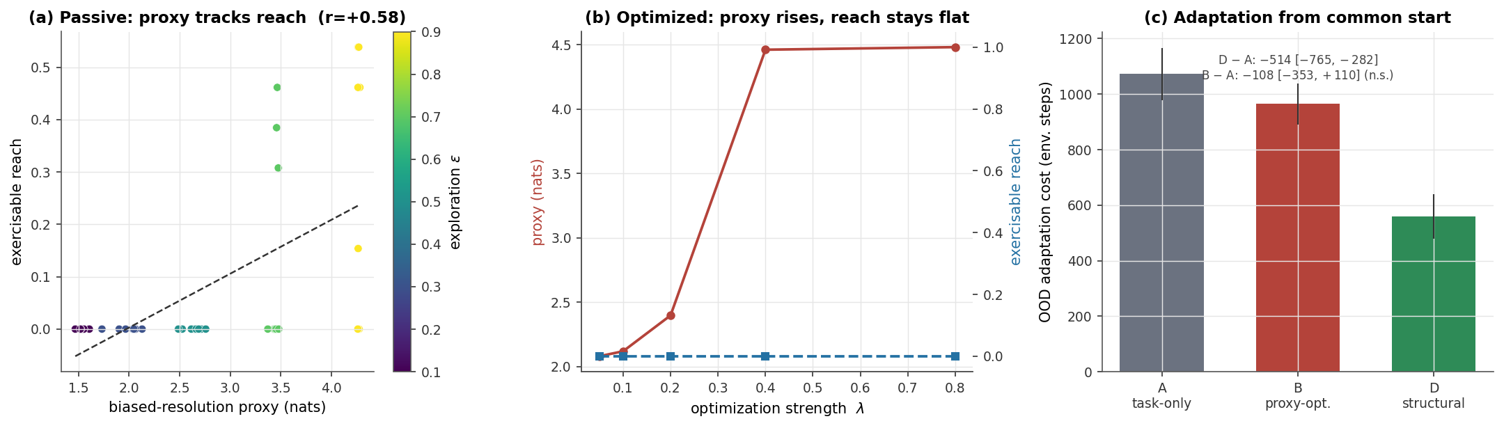
We use the proxy two ways. In the passive regime the agent is not rewarded for the proxy at all; we simply vary its exploration rate and read the proxy off as a diagnostic. Across exploration levels the proxy and exercisable reach rise together (Figure 1a): pooled across seeds the correlation is r = +0.63, and across the five exploration conditions' means it is +0.92. The coupling is genuine but it is a between-regime, common-cause effect — within a single exploration level the correlation is only +0.19 — because broader exploration lifts both the proxy and the agent's coverage of the periphery at once. As a sensor, read across natural variation, the proxy is informative about reach.

In the objective regime an arm (B) is rewarded for raising the same proxy, with the reward weight λ swept upward. The proxy climbs from roughly 2 to 4.5 nats while exercisable reach stays flat at zero across the entire sweep (Figure 1b). The optimizer discovers that the cheapest way to raise a proxy resolved finely in the meadow and coarsely at the edge is to spread through the meadow; the single coarse far-category offers no gradient worth the bottleneck's cost. The same proxy that tracked reach when observed is silent about reach when optimized. A structural arm (D), which never optimizes the proxy but simply begins episodes from states drawn across the whole space, attains full exercisable reach from the common start — at a lower proxy score than the optimized arm.

Two controls locate the phenomenon rather than merely exhibiting it, and are reported in Section 8: a proxy over a feature space the meadow already saturates is never coupled to reach even passively, so its failure under optimization would prove nothing; and a proxy that is count-based novelty over the full state stays coupled even when optimized, because it is close to a sufficient statistic for reachability. The decoupling of interest requires a proxy that is both passively informative and lossily resolved — neither an irrelevant proxy nor a near-sufficient one qualifies.

Finally we test what the retained structure is worth after a shift. Holding out the trained transition models, we move the goal into the far region and measure the environment steps each arm needs to first reach it from the common start, planning with its retained model (Figure 1c). Structural exposure adapts in roughly half the steps of the task-only baseline (559 vs 1073); the bootstrap 95% interval for that difference is [−765, −282] and for structural-versus-optimized [−611, −191], both clear of zero. The optimized arm, however, is statistically indistinguishable from the baseline — its interval, [−353, +110], spans zero — despite carrying a far higher proxy score. Optimizing the proxy thus buys no reliable adaptation advantage while destroying zero-shot reach; structural exposure buys the advantage without touching the proxy.

Figure 1. Experiment 1: the biased-resolution proxy tracks exercisable reach as a sensor but not as an objective. (a) Passive regime — across five exploration levels (colour, ε from 0.1 to 0.9) the proxy and exercisable reach rise together; the pooled scatter and its fit show the between-regime coupling that makes the proxy informative when read off passively. (b) Objective regime — as the reward weight λ on the proxy is swept upward, the proxy climbs from roughly 2 to 4.5 nats (red) while exercisable reach stays pinned at zero (blue), the optimizer raising the score entirely within the finely resolved meadow. (c) Out-of-distribution adaptation cost from the common start after the goal is moved into the periphery: structural exposure (D) roughly halves the task-only cost (A), while the proxy-optimized arm (B) is statistically indistinguishable from the baseline despite its far higher proxy score. Bracketed values are bootstrap 95% intervals over twelve seeds.

4. Experiment 2: resolution and access cost as controlled variables

Experiment 1's tiling was drawn by hand, and a reasonable objection is that its coarse periphery is the modeller's artifact. Experiment 2 answers by making the tiling the independent variable. We split the peripheral region into a controllable number of categories, k_far — its resolution — while holding the meadow at a fixed thirteen, and we impose a per-step access cost c_b on movement within the periphery, a surrogate for how expensive the margin is to reach. Arm B optimizes the resulting proxy at a fixed optimization strength; we record exercisable reach, the proxy, and task competence in every cell of the k_far × c_b grid.

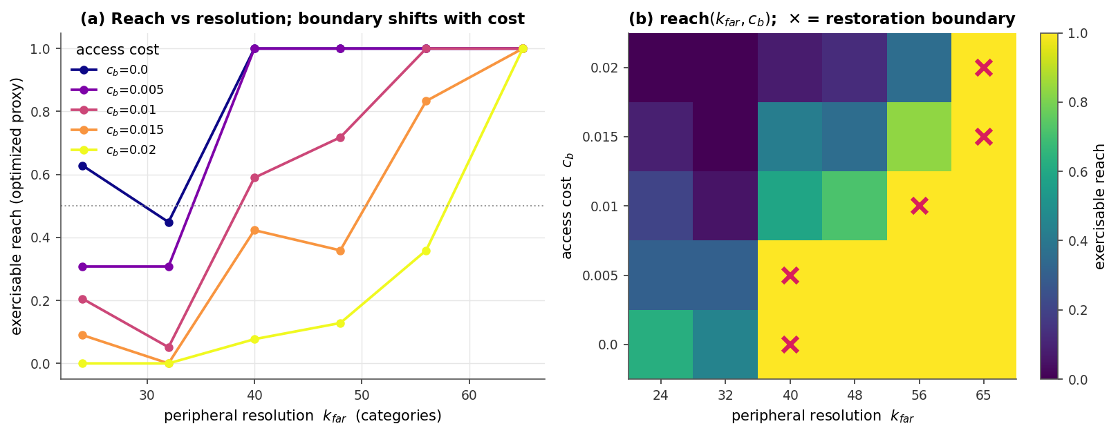
Reach rises with peripheral resolution at every cost, and rising cost pushes the recovery toward finer resolution (Figure 2). Reading the restoration boundary as the smallest k_far at which reach reaches 0.9, it moves from 40 categories at zero cost, to 40 at c_b = 0.005, to 56 at 0.01, to the full 65 at 0.015 and above. The complementary cut is equally clean: at fixed resolution k_far = 48, reach falls 1.00 → 1.00 → 0.72 → 0.36 → 0.13 as cost climbs. The observer must resolve the periphery finely enough relative to its access cost for the optimizer to find it worth reaching.

Figure 2. Experiment 2: peripheral resolution and access cost as controlled variables. (a) Exercisable reach under optimization as a function of peripheral resolution k_far, one curve per access cost c_b; reach rises with resolution at every cost, and higher cost shifts the recovery toward finer resolution. (b) The same reach over the full k_far × c_b grid (yellow = full reach, dark = none); crosses mark the restoration boundary, the smallest resolution at which reach reaches 0.9 for each cost. The boundary moves to higher resolution as cost rises, from additive main effects rather than a multiplicative interaction; away from the boundary the scalar is clean, and near it category placement matters as much as count.

Three checks discipline the reading. First, the interaction: fitting reach to log₂(k_far), c_b, and their product gives strong main effects — resolution +4.7 [+3.8, +6.0], cost −264 [−350, −210] — but an interaction of +59 with interval [−50, +185], straddling zero and of the wrong sign for the intuitive "cost blunts resolution" story. The boundary shifts with cost from additive main effects alone; the paper claims additivity, not a multiplicative interaction. Second, the proxy: its raw value rises with resolution, but normalized against its own ceiling it is flat between 0.90 and 0.96 throughout, so the agent saturates whatever alphabet it is given and the raw rise is the growing ceiling, not more even exploitation. Third, competence: the agent solves its original task in all forty-two cells, so lost reach is never an artifact of a broken controller. A further cut on optimization strength shows that weak pressure fails independently of resolution — at low λ the proxy barely rises above baseline and reach is zero even at the finest periphery — so restoration requires both sufficient resolution and sufficient pressure.

One qualification the figure should not hide. Peripheral resolution behaves as a clean scalar only away from the boundary. In the transition zone the specific partition matters as much as the count: at one boundary cell, six random tilings of the periphery into the same number of categories produced reach from 0.03 to near one, with across-partition variation about five times the seed noise; at saturation the same tilings all give one. So k_far controls the saturated regime cleanly, and near the boundary it conflates category count with category placement. We therefore describe a cost-dependent restoration boundary, not a universal phase transition in a single scalar.

5. Experiment 3: the bias arises from the data

Both previous experiments impose the observer. The question that decides whether any of this matters is whether a representation learned from experience allocates its resolution the same way on its own. We stand in for a learned representation with a visitation-weighted k-means over states: given a fixed budget of categories, it places them where the data is dense and lets rarely visited states collapse into the nearest category. This is the faithful minimal form of "capacity follows the training distribution." We learn such a tiling from four data regimes — task-directed operation, passive broad exploration, structural random-spawn exposure, and a mixed blend — then use each learned tiling as the proxy and measure the exercisable reach obtained when it is optimized.

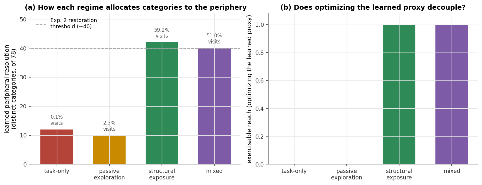
The result is stark and one-directional (Figure 3). At a budget of 78 categories, task-directed operation places only 0.1% of its visits beyond the bottleneck; the learned observer spends 72 of its 78 categories on the meadow and twelve on the periphery, and optimizing that learned proxy yields zero exercisable reach. Passive exploration barely helps — it lifts peripheral coverage to 2.3%, still leaves the far region compressed into ten categories, and still yields zero reach — because the bottleneck means undirected noise almost never assembles the sequence that reaches the far region. Only structural exposure, which samples the periphery directly (59.2% of visits), allocates enough peripheral categories (42) for the learned proxy's optimization to preserve full reach; the mixed regime (51.0%, 40 categories) does the same. The qualitative split is robust across category budgets of 52, 78, and 104.

Figure 3. Experiment 3: the resolution bias arises from the data rather than the modeller. (a) Effective peripheral resolution — distinct learned categories touching the periphery, of a budget of 78 — under four data regimes, with each regime's share of visits beyond the bottleneck annotated; task-directed and passive-exploration data spend almost all resolution on the meadow and fall below the Experiment 2 restoration threshold (dashed), while structural and mixed exposure clear it. (b) Exercisable reach obtained when each learned proxy is optimized: zero for the task-only and passive representations, full for the structural and mixed ones. Broader exploration does not repair the bias; exposure that samples the periphery does.

The counted "peripheral resolution" slightly overstates how well the far region is resolved, and the discrepancy is itself informative. At a budget of 104 the task-directed learner nominally places thirty categories in the periphery yet still yields zero reach, because those categories fall on the near periphery it occasionally clips while the far region behind the bottleneck collapses to essentially one. Exercisable reach, not the category count, is the quantity that reports the outcome, and it is unambiguous: the resolution bias of Experiments 1 and 2 is not a modelling choice but a consequence of the data a task-centred agent generates, and only exposure that changes that data — not more exploration within it — repairs it.

6. The mechanism: an excitation-starved observer

The three experiments describe one object from three angles, and Section 5 lets us finally say what that object is. It is not "a bad metric." It is a feedback loop between what a system does and what its measuring apparatus can see — a loop that is self-reinforcing and spatially structured, and that a control engineer would recognise on sight as a persistent-excitation failure folded into an objective.

Recall the identification problem underneath the whole paper. A learned observer — here a visitation-weighted clustering, in a real system any representation trained on operational data — allocates its finite resolution to the regions of state space its training data actually populates. Richly sampled regions are finely distinguished; barely sampled regions are compressed into a residual category, because a representation cannot preserve distinctions it has had little opportunity to observe. In control terms: poorly excited modes are weakly identified. This is not a defect of the learner. It is what "learned from data" means.

Now close the loop (Figure 4). A task-centred controller keeps the central region persistently excited and the periphery essentially dark; in the toy, task-directed operation places roughly 0.1% of its visits beyond the bottleneck. The observer trained on that trajectory therefore resolves the centre finely and the far periphery into almost nothing — at a budget of 78 categories, twelve touch the periphery and, functionally, none reach the far region. A diversity proxy built on that observer can be maximised entirely within the centre: there are many cheap central distinctions to spread across and almost no represented distinctions at the edge, so the metric offers no reward for the expensive traversal outward. An optimiser following that reward stays central. Staying central keeps the periphery unexcited, which keeps it coarsely represented, which keeps the metric silent about it. The loop has closed on itself.

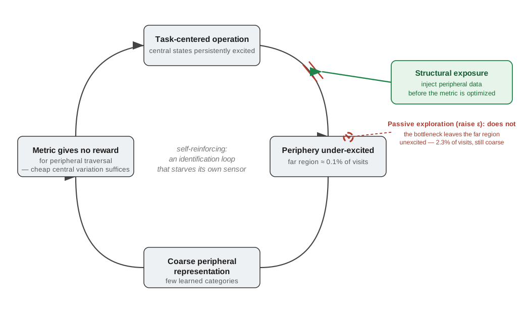
Figure 4. The excitation-starved observer as a positive feedback loop: task-centred operation leaves the periphery under-excited, a representation learned from that trajectory resolves the periphery coarsely, and a proxy built on it offers no reward for peripheral traversal — so the optimizer stays central, keeping the periphery unexcited. Passive exploration does not break the loop (the bottleneck leaves the far region at ~2.3% of visits); structural exposure, injected before the metric is optimized, does.

The consequence is worth stating in the metric's own terms: optimising the observer removes the very incentive that would have excited the region the observer cannot see. The sensor's blind spot is not a fixed property of the environment; it is produced, and then maintained, by the closed loop. This is the sense in which the failure is sharper than ordinary Goodhart. Ordinary Goodhart says an optimised proxy diverges from its target. Here the proxy also acts to preserve its own divergence: optimising it suppresses the excitation that would have corrected it. The corruption of the sensor, established for governance metrics in earlier entries in this series, is here shown to be spatially organised by excitation and self-amplifying rather than static.

Two features of this loop carry the paper's weight.

First, it is endogenous. Section 4 had to draw the coarse periphery by hand, and a sceptic could dismiss the effect as an artifact of a chosen tiling. Section 5 removes that objection. Nobody assigned the periphery twelve categories — the task-centred data distribution did, and it did so robustly: the qualitative outcome, task-centred and passive regimes decoupling while structural and mixed regimes restore reach, holds across representational budgets of 52, 78, and 104 categories. The bias is manufactured by ordinary operation, not by the modeller.

Second, and less obvious, the loop is not broken by exploring harder. The intuitive fix — inject noise, raise the exploration rate, "encourage more variation" — fails. Passive broad exploration lifts peripheral coverage only from 0.1% to 2.3%, still far too little: with a bottleneck between centre and periphery, undirected noise almost never assembles the specific sequence that reaches the far region, so the learned representation stays coarse and exercisable reach stays at zero. What breaks the loop is structural exposure — training data that samples the periphery directly, independent of the task-directed policy (in the toy, episodes begun from states drawn across the whole space). That regime lifts peripheral coverage to roughly 59%, so the learned representation resolves the far region it now actually visits, and exercisable reach returns to one. The distinction separates two governance instincts that sound alike: stimulate more activity versus guarantee observation of the margin. Only the second changes the data distribution upstream of the metric, and in the toy only the second works.

One honesty note the diagram should not paper over. "Peripheral resolution," counted as distinct categories touching any peripheral cell, slightly overstates how well the far region is resolved: a learner spends a few categories on the near periphery it occasionally clips while collapsing the far region behind the bottleneck into essentially one. At a budget of 104 categories the task-centred learner nominally places thirty categories in the periphery yet still yields zero exercisable reach, precisely because those categories sit near the boundary rather than at the far goals. Exercisable reach — planning and executing access from the common start — not the category count, is the quantity that reports the loop's outcome. The count is a diagnostic, and it must be read regionally.

7. A governance hypothesis (stated as hypothesis)

The gridworld proves nothing about any institution. What it supplies is a mechanism precise enough to state as a falsifiable prediction, and the translation, together with its limits, should be explicit before the claim is made.

The mapping is direct. Central, richly excited states correspond to the forms of activity an institution routinely performs and therefore routinely records: incumbent programmes, standard providers, applicants who arrive through established pathways. Peripheral, costly states correspond to genuinely different alternatives outside those pathways — unconventional providers, models that fit no existing certification category, populations the institution rarely reaches. An administrative representation — the schema of categories, codes, and performance histories through which an institution "sees" its domain — is a learned observer in exactly the sense of Section 6: its resolution follows the data its own operations generate. It will resolve incumbent-compatible forms finely and compress peripheral alternatives into coarse residual classes, not by anyone's intent but because that is where the data is.

The failure appears at the next step: when allocation is tied to a diversity or pluralism score computed within that representation. The prediction is that such a system generates abundant measurable variety inside the incumbent space — many finely distinguished options that are all mutually near — while the score stays insensitive to the disappearance of costly, genuinely distinct alternatives it never resolved. The metric looks healthy while the reachable set of real alternatives contracts, and optimising the metric, by the loop of Section 6, further starves the observation that would have revealed the contraction.

Stated as a testable claim for the Governance as Engineering programme:

Task-centred administrative data allocates finer categorical resolution to incumbent-compatible forms than to peripheral alternatives; tying resource allocation to diversity measured within that representation amplifies the asymmetry over time; and the amplification is arrested only by structurally guaranteeing observation of the periphery — randomised audit, mandated field presence, distributed local sensing — introduced upstream of the point at which the indicator becomes an allocation target.

Each clause is separately checkable against administrative records: the resolution asymmetry by auditing categorical granularity across incumbent versus peripheral cases; the amplification by tracking that asymmetry after a metric is tied to funding; the intervention by comparing agencies that do and do not mandate peripheral observation. That is the shape of an empirical study; the toy's role is only to say which quantities to measure and why they should move together.

The corresponding design guidance is the negative result made positive, and it inverts a common reflex. The instinct to preserve institutional diversity by rewarding diversity — scoring it, ranking it, funding against it — is precisely the move Section 6 identifies as self-defeating, because it optimises an observer whose blind spot it has not first repaired. The instinct the toy supports instead is unglamorous: spend the effort on observation of the margin rather than on the incentive, and spend it before the metric is coupled to consequences. An institution that guarantees it will keep sampling the alternatives outside its normal pathways preserves the option to fund them; an institution that merely scores the diversity it already sees will, under optimisation, keep the diversity it already sees.

Three limits bound the claim and should travel with it. The toy is deterministic, single-mapped, and free of strategic agents, so it speaks to the observational mechanism and not to gaming by the observed. Its "structural exposure" preserves only alternatives the designer already knows to sample — random restart across a known state space — and therefore says nothing about preserving alternatives no one has yet imagined, which is the harder governance problem and remains open. And the mapping from a visitation-weighted clustering to any particular administrative representation is an analogy, not an identity: the mechanism should generalise to any observer whose resolution follows its training distribution, but that is a claim to be tested across representations, not assumed.

8. What did not survive

The surviving claim is narrow, and its credibility rests largely on the breadth of adjacent claims that were tested and discarded. A diversity metric that fails under optimization is an easy thing to demonstrate badly — by choosing a metric rigged to fail, or by reading a general law off a single favourable plot. Most of the work in this paper went into refusing those demonstrations, and it is worth recording what was refused.

Two proxy designs were built and rejected before the one reported in Sections 3–5. The first, a proxy defined over a coarsened feature space that the central region already saturated, produced zero peripheral reach even without optimization — which means it was never a valid sensor of the latent property, so its failure under optimization would demonstrate nothing. The second, count-based novelty over the full state, remained coupled to exercisable reach even when optimized: rewarding visits to unvisited states is close enough to rewarding reachability that there was nothing left to corrupt. These two are not discarded prototypes but boundary controls. They locate the phenomenon: the interesting failure requires a proxy that is genuinely informative when observed passively and exploitable when optimized, and neither an irrelevant proxy nor a near-sufficient one qualifies. A single-run demonstration that skipped these controls would have been indistinguishable from a rigged one.

The interaction between resolution and cost, which both early verbal formulations of the conjecture asserted, did not survive its own formal test. The natural story — that access cost makes additional peripheral resolution less effective, a multiplicative interaction — was fit directly: strong main effects, resolution positive and cost negative with intervals well clear of zero, but an interaction coefficient whose bootstrap interval straddled zero and whose point estimate carried the wrong sign for the conjecture. On the logit scale the restoration boundary shifts with cost from the additive effects alone; no multiplicative interaction is needed or supported. The paper therefore claims additivity, and the "Cost–Resolution Conjecture" as first phrased is retired to that additive form. This is the clearest instance in the project of a formal analysis overruling a verbal one that had felt correct.

"Proxy inflation" was also weaker than it first appeared. Raw proxy entropy rises with resolution, but normalized against its own ceiling it is essentially flat, between 0.90 and 0.96 across the whole resolution range: the agent saturates whatever alphabet it is given, and the raw rise reflects the growing ceiling rather than more even exploitation. The correct statement is not that optimization inflates the proxy but that the agent maximally exploits the proxy at every resolution; what changes across conditions is the number of available distinctions, which is the manipulated variable itself.

The cleanest single knob of Experiment 2 turned out not to be clean. Category count sets the rough location of the restoration boundary, but near that boundary the specific partition — which peripheral cells share a category — matters as much as their number: at one transition cell, six random tilings of the periphery into the same number of categories produced reach ranging from 0.03 to near one, with across-partition variation roughly five times the within-partition seed noise. Away from the boundary, at saturation, geometry washes out. Peripheral resolution is thus a clean scalar only in the saturated regime; at the transition it conflates count with placement, and the "boundary" is partly a property of the tiling, not of its cardinality. The paper does not claim a universal phase transition in a single resolution scalar, and its figures are labelled accordingly.

Finally, the adaptation result was narrowed by its own statistics. Structural exposure reduces the cost of adapting to a shifted goal, significantly, relative to both the task-only baseline and the proxy-optimized arm. But the proxy-optimized arm is statistically indistinguishable from the baseline on adaptation — the bootstrap interval for that difference spans zero — despite a substantially higher proxy score. The defensible claim is therefore that optimizing the proxy buys no reliable adaptation advantage while destroying zero-shot reach, not that it actively degrades adaptation. The apparent improvement at one optimization strength was noise.

Each of these is a claim the evidence would have supported loosely and a stricter test removed. What remains after their removal is the spine of Sections 3–7, and it remains because these were tried against it and did not hold.

9. Limitations

The limitations fall into two kinds: those that bound what the result is about, and those that bound how firmly it is established. Separating them keeps either from being used to wave away the other.

On scope, the environment is a single deterministic gridworld with one bottleneck and one hand-defined peripheral region. Determinism means the observer's blind spot is produced purely by where the policy goes, with no stochastic dynamics complicating identification; a stochastic environment would add a second, orthogonal source of weak identification that this paper does not address. The single map means the specific numbers — coverage fractions, category counts, the restoration boundary — are properties of this geometry and carry no quantitative weight elsewhere; only the qualitative mechanism is claimed to travel. The peripheral region is defined by the modeller rather than discovered, which is appropriate for a controlled study but means the paper demonstrates the compression of a known periphery, not the detection of an unknown one.

The learning machinery is likewise minimal by choice. Tabular Q-learning was used so that a failure of exercisable reach could be attributed to the objective rather than to function approximation; a neural agent might interact with the mechanism in ways this design cannot see, and confirming that the effect survives function approximation is left to replication. The learned representation is a single instance, visitation-weighted k-means, chosen because its allocation of categories by data density is transparent and dependency-free. The mechanism it illustrates — capacity following the training distribution — is generic to representation learning under a distribution-averaged loss, but that generality is asserted here, not shown; a representation trained with a reconstruction, contrastive, or successor objective might allocate resolution differently, and Section 10 treats this as the first thing to test.

The structural intervention carries the most important scope limit, and it was flagged where it arose. "Structural exposure" here is random restart across the known state space: it preserves access to peripheral regions the designer already knows to sample. It therefore speaks to the preservation of enumerable alternatives and says nothing about preserving alternatives no one has yet conceived — the harder and more consequential governance problem, which this paper does not touch. Presenting random-start exposure as a general model of "keeping options open" would overreach in exactly the direction the paper is otherwise careful to avoid.

On confidence rather than scope, the seed counts are small. Saturated and empty cells are effectively deterministic across seeds, but the transition cells, where reach is near-bimodal across seeds, carry wide intervals at six seeds, and the boundary location within the transition zone is correspondingly uncertain. The partition-invariance check was run only at saturation and with a handful of tilings; the finding that geometry matters at the boundary is therefore established as a positive existence result — some partitions collapse reach — rather than as a characterized dependence. None of this changes the qualitative conclusions, but it bounds how sharply the boundary can be drawn, and the paper's language is kept correspondingly soft where these bite.

The final limit is the one that matters most for a Governance as Engineering paper and cannot be repaired within the toy: there is no institutional data here at all. The gridworld supplies a mechanism and a prediction. Whether any real administrative system exhibits the predicted resolution asymmetry, and whether tying allocation to a within-representation diversity score amplifies it, are empirical questions about institutions that only institutional data can answer. Section 7 is a hypothesis for exactly this reason, and should not be read as anything stronger until such data are brought to bear.

10. Future work

Three tests would materially strengthen the claim, in rough order of how directly they attack its weakest joints. The list is deliberately short. The failure mode this project spent most of its length escaping was the proliferation of plausible next questions; naming only the tests that can change a conclusion is itself part of the result.

The first is to replace the single representation-learner with several and place each against the ruler of Experiment 2. Train representations from the same four data regimes using a reconstruction autoencoder, a contrastive objective, and successor features, and for each measure the effective peripheral resolution allocated and the exercisable reach obtained when it is optimized. The question is no longer whether a learned representation compresses the periphery, but whether task-centred representation learning in general lands in the decoupling regime — and, sharply, where on the Experiment 2 resolution axis a naturally trained representation falls. If reconstruction and contrastive objectives place the periphery below the restoration boundary as weighted k-means does, the mechanism is a property of learning from operational data rather than of clustering; if they do not, the claim narrows to a class of representations, and the paper should say which.

The second is to vary the geometry the toy holds fixed. Multiple maps, multiple bottleneck placements, and stochastic transitions would separate the mechanism from the particular corridor used here, and would test the one prediction the paper makes structurally but has not swept: that traversal cost and bottleneck length raise the peripheral resolution required for restoration. Stochastic dynamics are the more important addition, because they introduce a second source of weak identification and would show whether excitation-driven compression and noise-driven compression add, interact, or mask one another. A goal-conditioned or empowerment-based measure of reach, rather than reachability of a fixed goal set, would further confirm that the finding concerns retained option value broadly, and not an artifact of the specific far goals chosen.

The third is the one the paper exists to motivate and cannot itself perform: a single real administrative case study testing the Section 7 prediction. Take one indicator regime in which resource allocation is tied to a measured diversity or pluralism score; audit the categorical granularity the administrative representation assigns to incumbent-compatible versus peripheral cases; and test whether that asymmetry widened after the metric was coupled to funding. A negative result would bound the mechanism's real-world relevance; a positive one would move it from analogy to evidence. Either outcome is more informative than further work inside the gridworld, which has now yielded what a gridworld can.

11. Conclusion

The paper began from a governance move — measure adaptive capacity, then steer by the measurement — and put to it the question a control engineer puts to any such loop: what does the sensor fail to see, and what does closing the loop do to that blind spot. The answer, in a minimal system, is specific and uncomfortable. A diversity indicator is an observer whose resolution is allocated by excitation. Task-centred operation excites the centre and starves the periphery; the observer therefore resolves the centre finely and compresses the periphery; and optimizing the resulting indicator rewards cheap central variation while leaving the periphery unreached — which keeps it unexcited, which keeps it compressed. The blind spot is not handed down by the environment but produced and maintained by the closed loop, and the act of optimizing the observer is precisely the act that suppresses the excitation which would have corrected it.

What gives the claim whatever weight it carries is less the favourable result than the sequence of unfavourable ones around it. The two boundary-control proxies fail for opposite reasons. The multiplicative interaction the conjecture wanted did not survive its own test. "Proxy inflation" turned out to be a moving ceiling. The clean scalar knob proved geometry-dependent at its boundary. The adaptation advantage vanished inside its own confidence interval. Each was a claim the evidence would have tolerated loosely and a stricter test removed, and what remains is narrow because of what was taken away: a mechanism, shown in one deterministic gridworld, by which a learned diversity metric decouples from the capability it names when it is optimized, together with a single intervention that repairs the decoupling by changing what the observer is permitted to see.

We have been careful not to inflate that residue into a law. The gridworld cannot show that any institution measures its options this way. It can show that the failure is mechanically possible, name the two quantities that govern it — how finely the periphery is resolved and how costly it is to reach — and predict how they should move together in a real administrative record. Whether they do is the empirical question Section 7 poses and Section 10 leaves open. The contribution is to have made that question precise enough to be worth asking, and to have shown that the intuitive remedy — rewarding measured diversity — is the one move that, under optimization, reliably fails. The remedy the mechanism points to instead is duller and prior: guarantee that the margin is observed before the metric is made to matter. An institution that keeps sampling the alternatives outside its own pathways keeps the option of using them; an institution that only scores the diversity already in view will, when pressed to optimize, keep exactly the diversity already in view.

Appendix A. Environment, agent, and hyperparameters

Environment. A 17×15 gridworld (interior 11×15) with the layout below, where S is the start, 1 the training goal (G1), # walls, g and 2 the thirteen peripheral goals, the meadow occupying rows 1–7 and the periphery rows 8–15. A single gap in row 8 (the bottleneck) and a single door into the enclosed far region are the only routes to the periphery.

###############
#.............#
#.............#
#......1......#
#.....S.......#
#.............#
#.............#
#.............#
#######.#######
#.............#
#.###########.#
#.#gg.....gg#.#
#..gg..2..gg#.#
#.#gg.....gg#.#
#.###########.#
#.............#
###############

Four deterministic actions (up, down, left, right); walls block; the transition is otherwise identity-plus-move. Central and peripheral regions are defined by row: meadow rows ≤ 7, periphery rows ≥ 8.

Agent. Tabular Q-learning, γ = 0.99, α = 0.5, ε-greedy behaviour with ε = 0.15 unless swept, 4000 episodes of up to 120 steps, fixed start unless the structural regime is used. Base reward is −0.01 per step and +1 at G1; Experiment 2 adds −c_b per step taken in the periphery. Tabular (rather than a neural agent) is a deliberate choice so that any loss of reach is attributable to the objective rather than to function approximation.

Proxy and its optimization. The proxy is the Shannon entropy (nats) of the agent's visitation distribution over tiles. The biased tiling resolves the meadow at m_meadow categories (one per cell in Experiment 1; m_meadow = 13 in Experiment 2) and the periphery at k_far categories (one in Experiment 1; swept in Experiment 2), assigned by contiguous split unless the random-partition control is used. Arm B adds an intrinsic reward λ_t · (count(tile) + 1)^(−1/2), where the count is cumulative and λ_t decays linearly to zero by 70% of training, so that the agent remains a competent solver of G1 (verified per condition).

Exercisable reach. After training, the agent's experienced transitions form a directed graph; a peripheral goal is exercisable iff a directed path to it exists from the common start using only experienced transitions. Because the environment is deterministic and the learned model is exact on experienced transitions, graph reachability from the start is equivalent to a plannable-and-executable route. Reach is the fraction of the thirteen peripheral goals so reachable.

OOD adaptation (Experiment 1). The goal is moved to a peripheral state and each arm adapts from the common start by Dyna-Q warm-started with its retained transition model (planning budget 10 backups per real step, ε = 0.2, step budget 20000). The reported cost is the number of real environment steps to first reach the shifted goal.

Structural regime. Episodes begin from states drawn uniformly across the free state space rather than from the fixed start; the task reward is unchanged and the proxy is not optimized.

Learned representation (Experiment 3). Visitation counts are collected under each data regime (task-only ε = 0.15 from the fixed start; passive ε = 0.9; structural uniform-random start; mixed alternating), then a weighted k-means (weighted k-means++ initialization, up to 60 Lloyd iterations) over cell coordinates with weights equal to visitation counts produces K category labels. The labels become the tiling; effective peripheral resolution is the number of distinct labels among peripheral cells. K ∈ {52, 78, 104} was tested; the main figure uses K = 78.

Seeds. Six seeds per condition in the resolution sweep and Experiment 3; twelve in the exercisable-reach and adaptation runs of Experiment 1; eight in the regenerated passive/optimization figure panels. Saturated and empty conditions are effectively seed-invariant; transition conditions are not, and their intervals are reported accordingly.

Appendix B. Reproducibility manifest

Each row lists the artifact that produces a claim or figure, the cache it reads or writes, and the command. All scripts are pure Python over NumPy, SciPy, and Matplotlib; no network access or GPU is required, and all randomness is seeded.

Two reproducibility notes belong in the record. The resolution sweep is time-boxed and resumable: paper_xxiv_possibility_resolution_sweep_v2.py <seconds> fills as many cells as fit before exiting and can be re-invoked until the cache is complete, after which --plot tabulates and renders. And an earlier version of the sweep script did not reproduce its reported numbers — it omitted the m_meadow setting and used a coarser cost grid than the narrative described; the discrepancy was caught by re-running the shipped artifact and is corrected in the version listed here. The manifest exists so that this class of error is caught by construction rather than by luck.

Appendix C. Statistical methods

Normalized entropy. To separate a larger representational alphabet from more even exploitation of it, the raw proxy H is reported alongside H_norm = H / log(m_meadow + k_far), its value as a fraction of the maximum entropy attainable at that resolution. Across the Experiment 2 grid H_norm lies between 0.90 and 0.96, indicating near-saturation of the available alphabet at every resolution; the rise in raw H therefore reflects the growing ceiling rather than increasing evenness.

Interaction model. Seed-level exercisable-reach fractions (successes out of thirteen goals) are modelled as binomial with a logit link and linear predictor β₀ + β₁ log₂(k_far) + β₂ c_b + β₃ [log₂(k_far) · c_b], predictors centred. The fit is by maximum likelihood (BFGS on the binomial negative log-likelihood); confidence intervals are obtained by resampling the six seeds within each cell (400 bootstrap replicates) and refitting. The reported estimates are β₁ = +4.7 [+3.8, +6.0], β₂ = −264 [−350, −210], and β₃ = +59 [−50, +185]. The main effects are strong and of the expected sign; the interaction interval straddles zero with a point estimate of the wrong sign for a "cost blunts resolution" account, so the paper claims additive, not multiplicative, effects. The per-goal outcomes within a seed are not independent, so the binomial intervals should be read as approximate; a hierarchical per-goal model is noted in Section 10 as the sharper analysis.

Adaptation bootstrap. For the OOD-adaptation comparison, pairwise differences in mean step-cost between arms are bootstrapped over the twelve seeds (10,000 replicates, percentile intervals): D − A = −514 [−765, −282], D − B = −406 [−611, −191], B − A = −108 [−353, +110]. No seed in any arm reached the step budget, so the means are uncensored and the comparison is not distorted by a cap.

Partition variation. In the transition-zone geometry test, across-partition dispersion is the standard deviation of per-partition mean reach across random tilings of fixed cardinality, compared against the mean within-partition seed standard deviation. At the boundary cell these are ≈ 0.35 versus ≈ 0.07; at saturated cells the across-partition dispersion collapses to near zero.