Closure–Adaptation Dynamics

Abstract

This paper introduces a minimal dynamical model of institutional closure and adaptation under uncertainty, as a contribution to Governance as Engineering. The model consists of five coupled variables: actual unresolved environmental uncertainty, boundary strength, trust capacity, exploratory capacity, and boundary permeability. The central distinction is between boundary strength and boundary quality: a boundary may be strong but permeable, reducing felt uncertainty while preserving information flow, or strong and impermeable, reducing felt uncertainty while destroying the capacities for learning and adaptation.

The model exhibits a robust set of behaviours. It is bistable across a wide parameter range: the same environment can support an open, high-trust, exploratory regime and a closed, low-trust, non-adaptive regime, with the outcome determined by initial conditions. It displays hysteresis: the threshold for collapse into closure is higher than the threshold for recovery from closure, so systems that have closed require substantially safer conditions to reopen. Under moderate perceptual noise, the open regime is stable because the slow permeability variable buffers transient fear spikes; but at high stakes and high noise, a residual probability of noise-induced tipping appears. In a two-population extension, populations with different histories can stably polarize into open and closed regimes under identical external conditions, and a severe closure event in one population can cascade to the other through the shared increase in actual uncertainty.

The paper also tests a simple governance intervention: a constitutional minimum on boundary permeability—a floor that cannot be breached even during a crisis. For the tested shock parameters, a floor of $P_{\min}=0.4$ completely prevents the permanent closure that otherwise follows a combined stakes-and-opacity shock. The mechanism is the preservation of the trust–exploration loop through the crisis. This result gives formal support to the idea that transparency protections are not merely normative preferences but load-bearing design requirements for adaptive governance.

The formal results are reported as [R within model]: they hold for the stated equations, parameter values, and numerical envelopes, and claim nothing directly about real institutions. The governance interpretations—concerning the design of slow protections, minimum permeability floors, and the public-good character of openness in coupled systems—are offered as [IP]. The model is deliberately minimal, and its limitations are stated explicitly. Its purpose is to isolate a small set of feedbacks that are plausible, robust, and consequential, and to provide a diagnostic lens for institutional rigidification under uncertainty.

1. Introduction

Governance as Engineering treats governance systems as feedback controllers embedded in environments they can observe only partially, act upon with delay, and model with bounded representational capacity. A central claim of the series is that many institutional failures are architectural rather than behavioural: they arise not from insufficient competence or will but from structural mismatches between how a system senses, decides, and acts, and the dynamics of the world it seeks to govern. Paper XII established that boundary selection is an independent design variable and that the pooling paradox makes the trade-off between integration and autonomy inescapable for any fixed boundary. Paper XV showed that adaptive capacity is gated by the slowest stage of the sense–learn–execute loop. Paper XVI identified the source-term structure underlying the erosion of exploration. Paper XVIII proved that under persistent learning, no fixed decomposition of jurisdiction and environment survives, and that a controller can weld its own boundary shut past a reflexivity threshold.

This paper extends that line of work by asking a question the earlier papers left implicit: What happens when the boundary itself is not fixed, but driven by felt uncertainty, and when its quality—not only its strength—is allowed to degrade under stress? We introduce a minimal dynamical model in which five variables co-evolve: actual unresolved uncertainty $U$, boundary strength $B$, trust capacity $T$, exploratory capacity $E$, and boundary permeability $P$. The model is deliberately small, designed to capture qualitative mechanisms rather than to reproduce any specific institution. Its governing equations are given in Section 2.

The model produces a coherent set of phenomena that together constitute a formal account of institutional rigidification under uncertainty:

• Bistability. For a wide range of parameters, the same environment supports two stable equilibria: an open regime with low boundaries, high trust, and high permeability, and a closed regime with maximal boundaries, near-zero trust, and low permeability. Initial conditions decide which regime is reached.
• Hysteresis. The thresholds for collapse into closure and recovery into openness differ: a system that has closed requires substantially safer conditions to reopen than a system that was never closed.
• Noise-induced tipping. Moderate perceptual noise does not disturb an open system under most conditions, but near the separatrix between attractors it can trigger a permanent transition to closure.
• Cascade collapse. In a two-population extension, a shock that drives one population into closure can raise the shared uncertainty burden on the other sufficiently to drag it into closure as well, even if it was not directly shocked.
• A critical transparency floor. A constitutional minimum on boundary permeability—a value that cannot be violated even during a crisis—prevents the closed attractor from locking in. In the model, a floor of $P_{\min} \approx 0.4$ is sufficient to guarantee recovery after a severe combined shock, while lower floors result in permanent closure.

These results connect directly to several earlier papers. The model can be read as a dynamic extension of Paper XII: boundaries are no longer chosen once but emerge from an ongoing trade-off between felt uncertainty reduction and adaptation loss. It also gives a concrete mechanism for the adaptation bottleneck of Paper XV, because the slow permeability variable acts as a second, slower loop that can throttle the sense–learn–execute cycle even when the fast variables are functioning. The model instantiates the source-term structure of Paper XVI: trust and exploration persist only through a source term that the boundary dynamics can destroy. And the combined shock experiment produces a locked state closely analogous to the boundary welding described in Paper XVIII, but through fear and opacity rather than through the controller's own learning dynamics.

The contribution of this paper is therefore not a new fundamental law, but a minimal model that ties together several previously separate threads into a single dynamical system. It shows that the boundary–trust trade-off, the adaptation bottleneck, the exploration-source-term structure, and the boundary-welding phenomenon can all be seen as consequences of one underlying closure–adaptation dynamics.

The paper is organised as follows. Section 2 defines the model and interprets each term in governance language. Section 3 derives the fast–slow structure and the conditions for bistability. Section 4 reports systematic phase diagram results and quantifies the robustness of the closure trap. Section 5 presents stochastic simulations and the residual fragility of the open state. Section 6 extends the model to two coupled populations and demonstrates polarisation and cascade collapse. Section 7 introduces the permeability-floor intervention and identifies the critical threshold. Section 8 discusses design principles, limitations, and open questions. Section 9 concludes.

All simulation results in this paper are numerical and should be read as [R within model]: they hold for the stated parameter envelopes and initial conditions, and claim nothing directly about real institutions. The governance interpretations that follow from them are [IP], in keeping with the series' discipline that formal models earn their keep as diagnostic lenses, not as empirical claims.

2. Model Definition and Governance Interpretation

We model a single governance system as a coupled five‑variable dynamical system. The variables are all dimensionless, bounded in $[0,1]$, and represent aggregate properties of the system rather than specific institutional features. The model is intended as a minimal abstraction: it captures feedback mechanisms that recur across many governance contexts without claiming to reproduce any particular institution.

2.1 State variables

The key distinction introduced in this model is between boundary strength $B$ and boundary permeability $P$. A boundary may be strong but permeable—for example, a quarantine that blocks physical movement but allows data and expertise to flow—or strong and impermeable—for example, a totalitarian information blackout. The variable $P$ captures this second dimension.

2.2 Auxiliary quantities

Define felt uncertainty $F$ as

$$F = \frac{s U}{(1+\lambda T)(1+\mu B)},$$

where $s$ is the stakes/uncertainty multiplier, and $\lambda,\mu>0$ are constants. Felt uncertainty is the system's internal experience of uncertainty. It is reduced both by trust $T$ and by boundary strength $B$, even if these do not reduce actual uncertainty $U$. This captures the familiar phenomenon that governments often build walls to make the world feel more predictable, rather than to make it more predictable.

Define the effective boundary suppression block $Q$ as

$$Q = (1-P)B.$$

This is the portion of boundary strength that actually suppresses trust and exploration. If permeability is high ($P \approx 1$), even a strong boundary does not damage the system's adaptive capacities. If permeability is low, the boundary becomes harmful.

2.3 Dynamical equations

The time evolution is given by:

$$\begin{aligned} \dot U &= n(1-U) - \alpha E (1-\beta Q) U, \\ \dot B &= \rho_B \, \sigma\!\big(k_B(F-\theta)\big) - d_B B, \\ \dot T &= \rho_T E (1-\beta_T Q) - d_T T - \gamma Q T, \\ \dot E &= \rho_E \, \sigma\!\Big( k_E \big( \frac{\alpha U}{1+\eta Q} - c_E \big) \Big) - d_E E, \\ \dot P &= \rho_P \left( 1 - \sigma\!\big( k_P(F-\theta_P) \big) - P \right), \end{aligned}$$

where $\sigma(z) = 1/(1+e^{-z})$ is the logistic sigmoid, and all parameters are positive.

Each equation has a direct governance interpretation.

Uncertainty equation. The term $n(1-U)$ represents the natural inflow of new disturbances, novelties, and environmental changes. The second term represents reduction of uncertainty through effective exploration. Boundaries reduce exploration's effectiveness if they are strong and opaque, via the factor $(1-\beta Q)$. Thus a closed system may be unable to reduce its actual uncertainty even if it feels secure.

Boundary equation. Boundary investment is driven by felt uncertainty: when $F$ exceeds a tolerance threshold $\theta$, the system builds boundaries. The sigmoid function $\sigma(k_B(F-\theta))$ is a smooth switch. Boundaries decay at rate $d_B$, representing institutional inertia and automatic sunset. The parameter $k_B$ controls how sharply the system responds to felt uncertainty.

Trust equation. Trust grows through exploration under open conditions, but only if the boundary is not too opaque. The term $\rho_T E (1-\beta_T Q)$ captures this: exploration builds trust when it is not blocked. Trust decays at rate $d_T$, and is further eroded by the boundary suppression block $Q$ through the term $-\gamma Q T$. Thus an opaque boundary actively destroys trust.

Exploration equation. Exploration is triggered when actual uncertainty is high relative to a cost threshold $c_E$, but is suppressed by opaque boundaries. The sigmoid $\sigma(k_E(\alpha U/(1+\eta Q)-c_E))$ captures the decision to explore: if the expected information gain $\alpha U$ exceeds the cost, exploration is active. Opaque boundaries raise the effective cost of exploration by a factor $1+\eta Q$. Exploration also decays at rate $d_E$, representing fatigue, budget cycles, or institutional forgetting.

Permeability equation. Permeability adapts slowly, with rate $\rho_P$, which is much smaller than the other rates. It tends toward a target value $1-\sigma(k_P(F-\theta_P))$: when felt uncertainty is low, the target is near 1 (openness); when felt uncertainty is high, the target is near 0 (opacity). The threshold $\theta_P$ is distinct from $\theta$, allowing the quality of boundaries to degrade before the system necessarily builds more of them. This slow equation is the model's representation of institutional trust erosion, media freedom, legal protections, and other slow-moving governance features.

2.4 Parameters and default values

For reproducibility, the parameter values used in the simulations are:

The time unit is arbitrary. Rates can be rescaled without changing the qualitative behaviour, provided the separation of timescales between $\rho_P$ and the other rates is preserved.

2.5 Scope and limitations

The model is not a calibrated empirical model. Its purpose is to expose qualitative mechanisms that are analytically and computationally tractable, and to generate testable hypotheses for more detailed institutional studies. The variables are aggregate constructs that condense many institutional features into single numbers, and the thresholds and sigmoids are deliberately sharp approximations to the continuous, heterogeneous processes in real governance systems. All numerical results should be read as [R within model], and any translation to real institutions as [IP].

With the model defined, Section 3 turns to the analytical structure of the fast–slow dynamics and the conditions under which bistability arises.

3. Analytical Structure: Fast–Slow Decomposition and Attractor Regimes

The model defined in Section 2 is five‑dimensional and nonlinear, but its behaviour can be understood through a standard fast–slow decomposition. The permeability variable $P$ evolves on a much slower timescale than $U,B,T,E$ because $\rho_P = 0.02$ while the other rates lie between $0.05$ and $0.55$. We therefore treat $P$ as a slowly varying parameter and analyse the four‑dimensional fast subsystem $(U,B,T,E)$ for fixed $P$. The full system’s trajectories then move along the equilibrium branches of this fast subsystem as $P$ changes.

This decomposition is not an approximation imposed for convenience; it reflects the substantive assumption that boundary quality changes more slowly than boundary strength, trust, or exploration. Constitutions, legal cultures, media environments, and institutional transparency norms are slower variables than the immediate policy responses they constrain.

3.1 Fixed points of the fast subsystem

For fixed $P$, the fast subsystem is:

$$\begin{aligned} \dot U &= n(1-U) - \alpha E (1-\beta Q) U, \\ \dot B &= \rho_B \, \sigma\!\big(k_B(F-\theta)\big) - d_B B, \\ \dot T &= \rho_T E (1-\beta_T Q) - d_T T - \gamma Q T, \\ \dot E &= \rho_E \, \sigma\!\Big( k_E \big( \frac{\alpha U}{1+\eta Q} - c_E \big) \Big) - d_E E, \end{aligned}$$

with $Q = (1-P)B$.

Because the sigmoids are steep ($k_B, k_E \gg 1$), the fast subsystem behaves approximately as a piecewise linear system with switching thresholds. Two stable fixed points emerge, corresponding to the open and closed regimes observed in simulation.

3.1.1 Closed attractor

Suppose $F > \theta$, so boundary investment is active, and suppose exploration is suppressed: $\alpha U/(1+\eta Q) < c_E$. Then:

• $\dot B = \rho_B - d_B B$, so $B \to \min(\rho_B/d_B, 1)$. With the default parameters, $\rho_B/d_B \approx 1.316$, so $B=1$ at saturation.
• $\dot E = -d_E E$, so $E \to 0$.
• With $E=0$, $\dot T = -d_T T - \gamma Q T$, so $T \to 0$.
• With $E=0$, $\dot U = n(1-U)$, so $U \to 1$.

Thus the closed fixed point is approximately

$$(B,T,E,U) \approx (1,0,0,1).$$

The felt uncertainty at this fixed point is

$$F_{\text{closed}} = \frac{s}{(1+\mu)}.$$

For the default parameters and $s=1.5$, $F_{\text{closed}} \approx 0.528$, well above $\theta=0.196$, so the boundary drive remains on. The exploration condition is also satisfied because $\alpha U/(1+\eta Q) = \alpha/(1+\eta(1-P))$, which is less than $c_E$ for a wide range of $P$. Thus the closed fixed point is self‑consistent.

Linearising around this fixed point shows that the eigenvalues are negative, dominated by the decay rates $d_B,d_T,d_E$ and the negative feedback in $\dot U$. The closed attractor is locally stable for all $P\in[0,1]$.

3.1.2 Open attractor

The open attractor is more delicate. It corresponds to a state where boundary investment is weak because felt uncertainty is below threshold, and exploration is partially active, keeping actual uncertainty moderate.

In the limiting case where $B$ is small and $P$ is sufficiently high, $Q \approx 0$. Then the equations reduce approximately to:

$$\begin{aligned} \dot U &= n(1-U) - \alpha E U, \\ \dot T &= \rho_T E - d_T T, \\ \dot E &= \rho_E \, \sigma\!\big(k_E(\alpha U - c_E)\big) - d_E E. \end{aligned}$$

If exploration is fully active ($E$ near its upper bound), the equilibrium values satisfy

$$U \approx \frac{n}{n+\alpha E}, \quad T \approx \frac{\rho_T E}{d_T}.$$

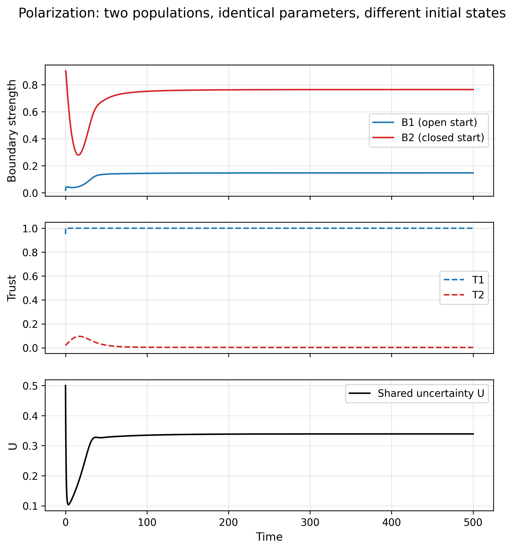
With the default parameters, the open state observed numerically has $B \approx 0.147$, $E \approx 0.179$, $T \approx 1.0$, $U \approx 0.34$, and $P \approx 0.70$. The small but nonzero $B$ is maintained by the boundary equation at a value where felt uncertainty is close to threshold $\theta$. The open fixed point is therefore a self‑regulating state: trust and exploration keep felt uncertainty low enough that boundary strength remains small, but not exactly zero.

The stability of the open fixed point depends on the trust–exploration loop. If $P$ is too low, $Q=(1-P)B$ becomes large even for small $B$, suppressing exploration and trust. This can destabilise the open state and push the system toward the closed attractor. The condition for stability is approximately that the effective boundary suppression $Q$ remains below a critical value $Q^*$, where

$$Q^* \approx \frac{\rho_T E}{\gamma T + d_T T} \quad \text{(for trust maintenance)}$$

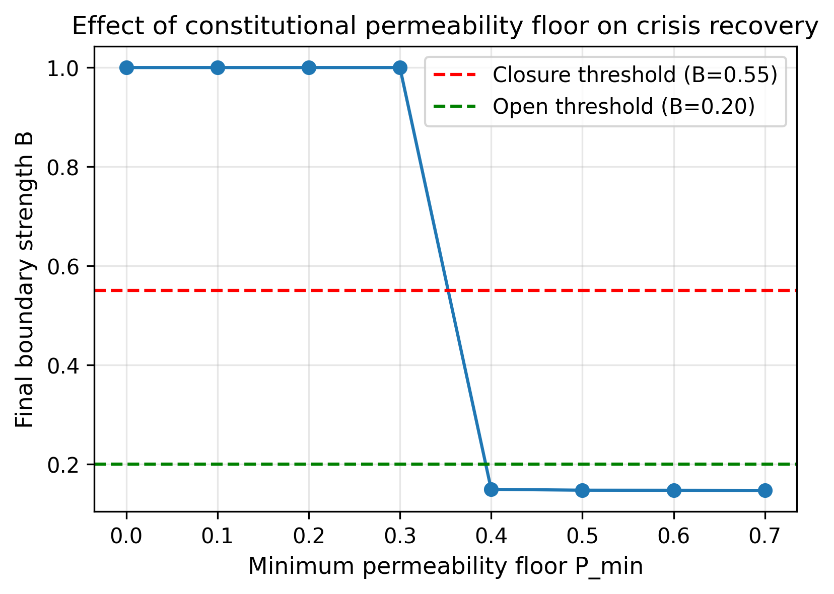
and similarly for exploration. In practice, the open attractor loses stability when $P$ falls below roughly $0.3$–$0.4$, depending on $s$ and $\theta$. This is consistent with the intervention threshold found in Section 7.

3.2 Bistability region

The coexistence of the open and closed fixed points for the same $P$ and $s$ defines the bistable region. It occurs when:

1. The closed fixed point exists and is stable: $s/(1+\mu) > \theta$.
2. The open fixed point exists and is stable: the trust–exploration loop is strong enough to keep felt uncertainty below threshold despite nonzero $B$.

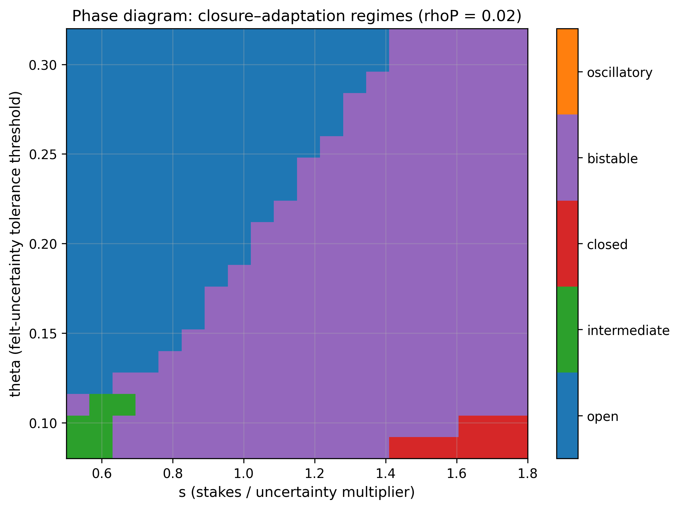
For fixed $s$ and $\theta$, the fast subsystem is bistable over an interval of $P$. In the default parameter regime at $s=1.5$, numerical continuation shows that both attractors exist for $P$ approximately between $0.1$ and $0.9$. Outside this interval, only one attractor remains.

The separatrix between the basins of attraction is not a simple line but a curved surface in the four‑dimensional fast state space. Its location depends on the history of the system, which is the origin of hysteresis in the full model.

3.3 Slow permeability dynamics and hysteresis

The slow equation for $P$,

$$\dot P = \rho_P \left( 1 - \sigma\!\big(k_P(F-\theta_P)\big) - P \right),$$

creates a positive feedback that reinforces whichever attractor the system currently occupies.

In the open attractor, $F$ is relatively low because $T$ is high and $B$ is small. With default parameters, $F_{\text{open}} \approx 0.077$, well below $\theta_P=0.15$. Therefore the target value $1-\sigma(k_P(F-\theta_P))$ is near $1$, and $P$ tends to increase toward $1$.

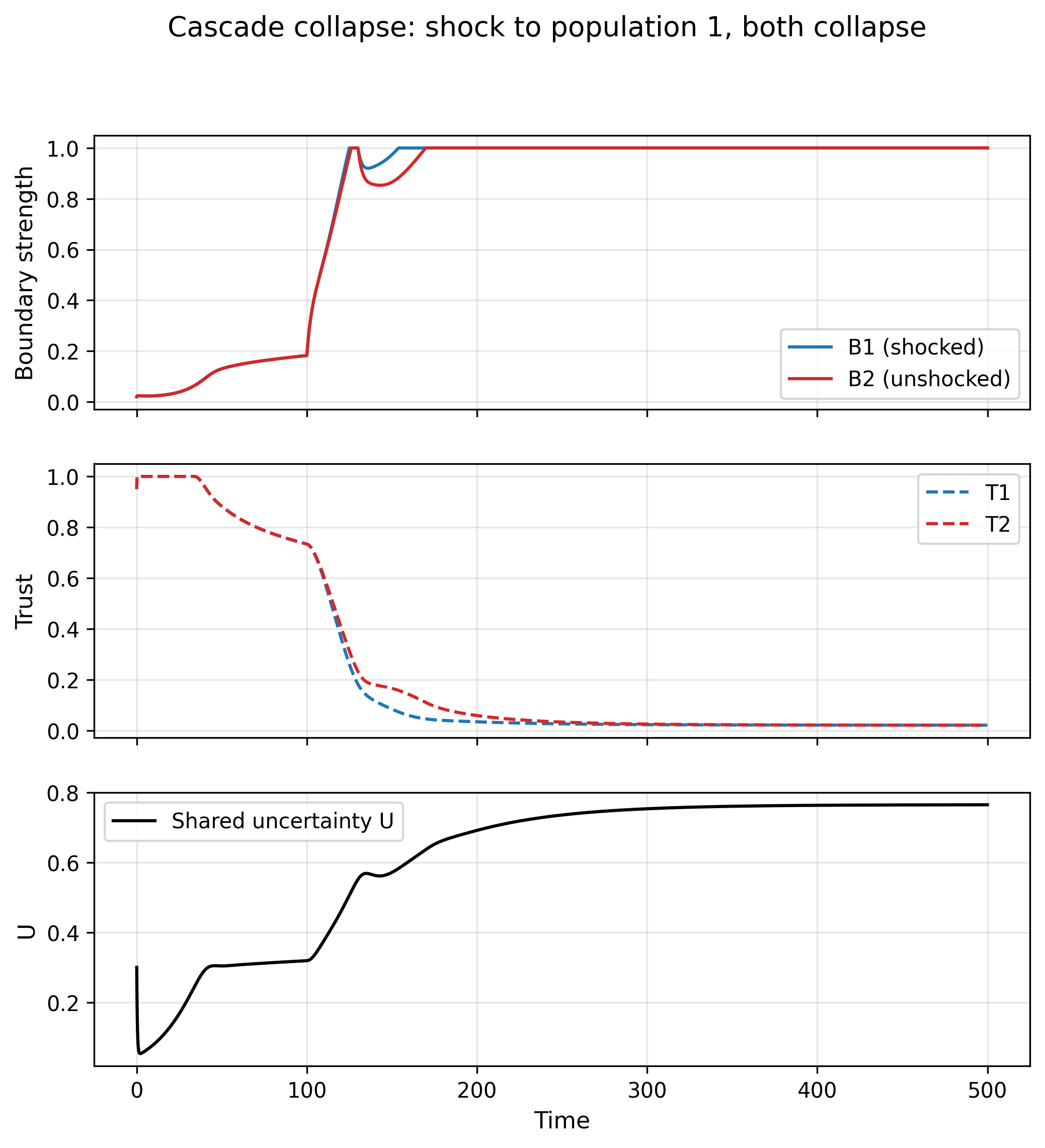
In the closed attractor, $F_{\text{closed}}$ is high (e.g., $0.528$ at $s=1.5$). The target value is near $0$, so $P$ tends to decay toward $0$.

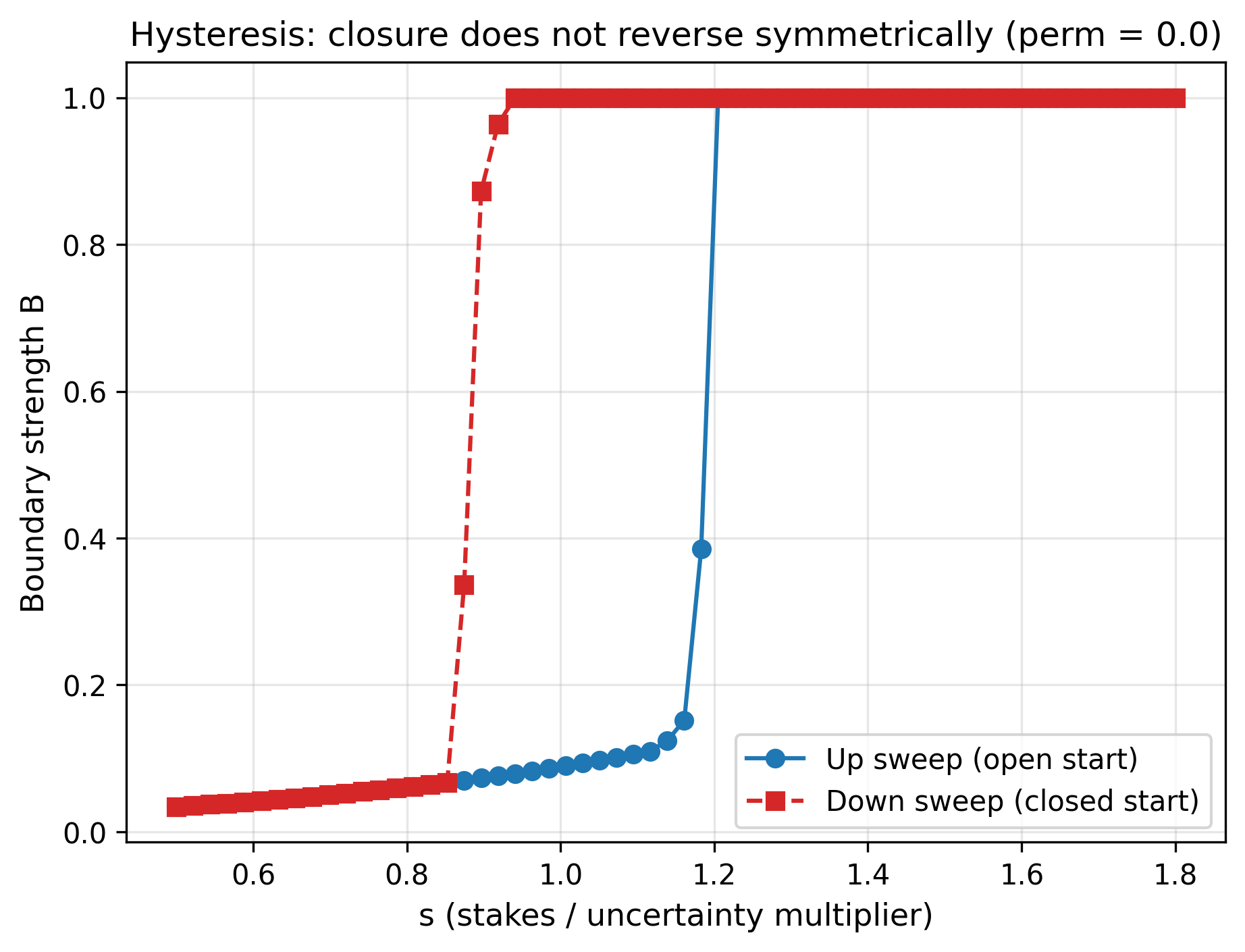
Thus the slow dynamics drive the system away from the separatrix: open states become more open, closed states become more closed. This is the mechanism of hysteresis.

When the system is on the open branch and external conditions worsen (e.g., $s$ increases), the open fixed point moves toward the separatrix. If the system crosses it, it falls to the closed branch. Once on the closed branch, $P$ begins to decay, further entrenching closure. To return to the open branch, external conditions must improve enough that the closed fixed point loses stability—but because $P$ has decayed, this requires much safer conditions than the original collapse point. This asymmetry is the hysteresis loop observed in the one‑dimensional sweeps.

3.4 Summary of analytical structure

The model possesses a clear fast–slow structure:

• The fast subsystem has two stable attractors: an open, high‑trust, high‑exploration state and a closed, zero‑trust, zero‑exploration state.
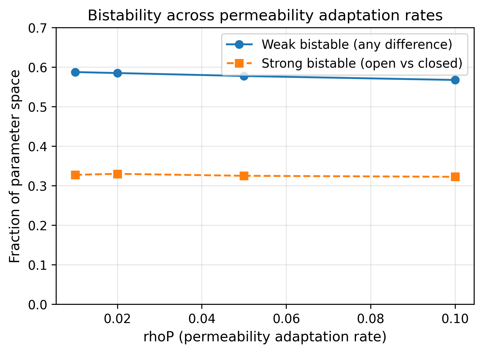
• Bistability occurs over a substantial range of $P$ and $s$, producing path dependence.
• The slow permeability variable amplifies whichever attractor the system occupies, creating hysteresis and institutional scarring.

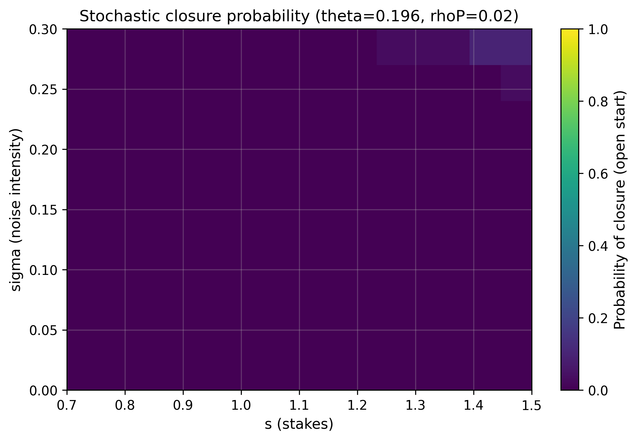
This structure is not assumed; it emerges from the interaction of boundary, trust, exploration, and permeability dynamics. Section 4 reports systematic simulations that quantify the extent of the bistable region across the parameter space, and Section 5 examines how noise interacts with this structure.

4. Phase Diagram and Robustness of the Closure Trap

The analytical structure of Section 3 indicates that bistability should occur for a range of parameters, but does not by itself establish how large or robust that range is. To answer this, we ran systematic simulations across a grid of stakes $s$, tolerance threshold $\theta$, and permeability adaptation rate $\rho_P$. The results show that the closure trap is a generic feature of the model, not an artefact of a narrow parameter choice.

4.1 Parameter sweep design

We swept the two parameters that most directly control the boundary–trust trade-off:

• $s$ (stakes / uncertainty multiplier): 20 values from $0.5$ to $1.8$
• $\theta$ (felt‑uncertainty tolerance threshold): 20 values from $0.08$ to $0.32$

For each of four values of the slow permeability adaptation rate $\rho_P \in \{0.01, 0.02, 0.05, 0.10\}$, we ran the deterministic five‑variable model from two initial conditions:

• Open start: $U=0.2,\ B=0.02,\ T=0.95,\ E=0.90,\ P=0.9$
• Closed start: $U=0.8,\ B=0.90,\ T=0.02,\ E=0.05,\ P=0.1$

Each simulation was integrated to $t=180$ with $dt=0.05$, and the final $B$ was averaged over the last 200 time steps. The final state was classified using the following rules:

• Open: $B_{\text{final}} < 0.20$
• Closed: $B_{\text{final}} > 0.55$
• Intermediate: $0.20 \leq B_{\text{final}} \leq 0.55$
• Oscillatory: standard deviation of $B$ over the tail $> 0.05$

Two notions of bistability were computed:

• Weak bistability: the two initial conditions lead to different final classifications (any difference).
• Strong bistability: the open start ends open ($B<0.2$) and the closed start ends closed ($B>0.55$).

The simulations are deterministic; all results reported here are [R within model] for the stated parameter grid and classification thresholds.

4.2 Qualitative structure of the phase diagram

The phase diagram for each $\rho_P$ shows the same three-region structure. Figure 1 shows a representative heatmap for $\rho_P=0.02$.

Figure 1: Phase diagram of the single-population model for $\rho_P=0.02$. Colors indicate the final regime classification from open and closed initial conditions, combined into weak bistability categories. The broad diagonal band shows the region of path-dependent institutional outcomes.

Three regions are evident:

1. Low stakes, high tolerance: the system is open regardless of initial condition. This region occupies the upper left of the $(s,\theta)$ plane, where felt uncertainty rarely exceeds the boundary threshold, and trust and exploration are self-sustaining.

2. High stakes, low tolerance: the system is closed regardless of initial condition. This region is small, occupying only about 2–3% of the tested grid. In these conditions, felt uncertainty is so high that even a well-trusted system cannot prevent boundary escalation.

3. A broad diagonal band of bistability: between these extremes, the same $(s,\theta)$ pair can support either the open or closed attractor, depending on initial history. This band is the model's representation of path-dependent institutional choice: two societies facing identical environmental conditions can end up in very different regimes because of differences in their starting trust, boundary strength, or permeability.

The transition from open to closed is not abrupt; it occurs through an intermediate zone where the open-start branch may settle at moderate $B$ before the closed-start branch becomes truly closed. This is why weak bistability covers a larger fraction of parameter space than strong bistability.

4.3 Quantifying robustness: weak and strong path dependence

Table 4.1 summarises the fractions of the tested parameter space in each regime, and Figure 2 shows the same information graphically.

Figure 2: Bistable fractions across permeability adaptation rates. Weak bistability (any difference in final classification) covers roughly 57–59% of the tested parameter space, while strong bistability (open vs closed) covers about 32–33%.

Table 4.1: Phase diagram fractions by regime and permeability adaptation rate

The main finding is that strong path dependence—the coexistence of a genuinely open and a genuinely closed outcome for the same parameters—occurs in roughly one third of the tested parameter space. Weak path dependence, including intermediate cases, covers nearly 60%. Only a small fraction of the grid forces closure unconditionally; most of the parameter space either remains open or is historically contingent.

This result answers the robustness question directly: the closure trap is not confined to a sliver of parameter space. It is a structural property of the dynamics across a wide range of stakes, tolerance levels, and permeability adaptation rates.

4.4 Effect of permeability adaptation rate

The summary also reveals a modest but consistent effect of $\rho_P$: as the permeability adaptation rate increases, the fraction of strongly bistable points declines slightly, from $0.328$ at $\rho_P=0.01$ to $0.323$ at $\rho_P=0.10$, and the fraction of both-closed points rises from $0.020$ to $0.030$. The mean collapse threshold also shifts downward by about $0.015$ over the same range (Table 4.2).

This suggests that faster permeability adaptation does not rescue the system. On the contrary, within the tested range, a more responsive permeability variable slightly increases the fragility of the open state. The likely mechanism is that when felt uncertainty rises, a faster $\rho_P$ allows $P$ to fall more quickly during a transient, deepening the suppression of trust and exploration before the system can recover. In governance terms, this corresponds to the danger of rapid institutional erosion under stress: legal and transparency protections that can be dismantled quickly are less protective than those that are slow-moving and therefore harder to degrade during a panic.

4.5 Hysteresis width

Table 4.2 reports the mean collapse and recovery thresholds computed from the phase diagram grid, together with the implied hysteresis width. Figure 3 shows a representative one-dimensional hysteresis loop for $\rho_P=0.02$, using the dynamic permeability model.

Figure 3: Hysteresis loop for boundary strength $B$ as stakes $s$ are slowly increased (up sweep, open start) and then decreased (down sweep, closed start) at $\rho_P = 0.02$. The separation between the branches shows that recovery requires substantially lower stakes than the collapse point.

Table 4.2: Mean thresholds and hysteresis width

The hysteresis width is positive for all tested $\rho_P$, confirming that the thresholds for collapse and recovery differ. A system that has fallen into the closed state requires conditions to become noticeably safer before it can reopen, compared with the conditions under which it originally collapsed. The width declines slightly with increasing $\rho_P$, consistent with the interpretation above: faster permeability adaptation narrows the gap, but does not eliminate it.

These aggregate numbers average over a range of $\theta$ and $s$, and should not be mistaken for a single universal threshold. The one‑dimensional hysteresis sweeps reported in earlier exploratory work show a sharper separation, with recovery occurring only after $s$ drops well below the collapse value. The aggregate table confirms the sign and robustness of the effect, while the scatter across $\theta$ is reported in the supplementary data.

4.6 Interpretation

The phase diagram results give formal content to the intuitive claim that civilisations systematically overproduce boundary structures when uncertainty exceeds their capacity for trust. The broad bistable region means that overproduction is not a universal law but a path-dependent possibility: for the same external conditions, one system may remain open while another locks down. The difference lies in the system's history—its accumulated trust, its initial boundary strength, and its permeability.

This is the dynamic analogue of the boundary–trust trade-off foreshadowed in earlier work. It gives a concrete mechanism for why high-trust and low-trust societies can persist side by side in similar environments, and why a crisis that pushes one society into closure may not affect another with a different initial configuration.

The next section turns to the role of noise. The phase diagram is deterministic; real governance systems face stochastic shocks, perceptual errors, and transient disturbances. We examine whether noise can move a system across the separatrix and how robust the open state is to such perturbations.

5. Stochastic Dynamics: Noise-Induced Tipping and Residual Fragility

The deterministic analysis of Sections 3 and 4 establishes that the open and closed regimes coexist across a wide parameter range, separated by a separatrix. In any real governance system, perception of the environment is noisy. Threat assessments are uncertain, information arrives with error, and transient shocks perturb the system away from its deterministic trajectory. This section examines whether such noise can move the system across the separatrix, converting a resilient open society into a permanently closed one.

5.1 Adding noise to felt uncertainty

We introduce noise into the model through the perceived felt uncertainty that drives boundary investment. The boundary equation becomes:

$$\dot B = \rho_B \, \sigma\!\big(k_B (F + \sigma \xi(t) - \theta)\big) - d_B B,$$

where $\xi(t)$ is Gaussian white noise with unit variance and $\sigma$ is the noise intensity. The other equations remain unchanged. This is a deliberately minimal modification: noise enters only through the perception of how uncertain or threatening the world is, not through the underlying state dynamics. It captures the idea that governments and institutions often overreact not because the environment has changed, but because their sensing apparatus has become noisy, biased, or unreliable.

All stochastic simulations use the full five‑dimensional model with slow permeability dynamics. Each run starts from the open attractor at the relevant $s$ and $\theta$, and noise is applied throughout the integration. The outcome is classified as “closed” if the final boundary strength $B$ exceeds $0.5$.

5.2 Stochastic sweep across stakes and noise intensity

We ran a Monte Carlo sweep over $s \in [0.7, 1.5]$ and $\sigma \in [0.0, 0.3]$, with $\theta$ fixed at $0.196$ and $\rho_P = 0.02$. For each parameter pair, 30 independent runs were performed, each starting from the open state and integrating for 200 time units. The probability of ending closed was recorded.

Figure 4 shows the full probability heatmap across the tested range.

Figure 4: Stochastic closure probability (open start) as a function of stakes $s$ and noise intensity $\sigma$, for $\theta = 0.196$ and $\rho_P = 0.02$. The open state is robust across most of the range; a small high-risk corner appears at high stakes and high noise.

The results are shown in Table 5.1 for selected $s$ and $\sigma$. The full grid is reported in the supplementary data.

Table 5.1: Probability of closure from an open start, selected parameter points

Two features stand out.

First, the open state is remarkably robust to noise across most of the tested range. Even at the highest stakes $s=1.5$ and moderate noise $\sigma=0.1$, not a single run out of 30 fell into closure. This is a consequence of the slow permeability dynamics: when a noise spike temporarily raises felt uncertainty, the system’s permeability $P$ does not immediately collapse. The trust–exploration loop remains intact, and the system returns to the open attractor once the spike passes.

Second, at the extreme corner of the parameter space—high stakes and high noise—a small but nonzero probability of closure appears. At $\sigma=0.2$ and $s=1.5$, 10% of runs ended closed; at $\sigma=0.3$ and $s=1.15$ or $1.3$, about 3% did. The standard deviation of final $B$ increases with noise, reflecting larger excursions toward the separatrix. Occasionally these excursions are large enough to cross it, after which the closed attractor takes over.

This residual fragility is important. It shows that the open state is not infinitely robust. There exists a finite band of conditions—high stakes and high perceptual noise—where random misperception can permanently tip a system into closure. Once tipped, the slow permeability dynamics drive $P$ downward, making the closed state self-reinforcing and recovery unlikely without a substantial improvement in conditions.

5.3 Comparison with fixed-permeability behavior

The contrast between this result and the behavior of a model with fixed, low permeability is instructive. In earlier exploratory work using a four‑variable model with $P$ held constant at a low value, noise of $\sigma=0.05$ was sufficient to produce 100% closure at $s=1.15$. The difference is entirely due to the slow permeability dynamics.

When $P$ is fixed low, a noise spike immediately increases felt uncertainty, which triggers boundary investment. The boundary then suppresses trust and exploration, raising actual uncertainty, which further raises felt uncertainty. The system falls into the closed attractor rapidly.

When $P$ is allowed to adapt, it acts as a buffer. A single noise spike cannot instantaneously destroy the system’s openness because $P$ changes only slowly. The system absorbs the perturbation and returns to the open state. Only sustained, large-amplitude noise at high stakes can overcome this buffer. This finding refines the earlier static analysis: boundary quality is not merely a design parameter; its temporal responsiveness is itself a key determinant of resilience.

5.4 Institutional interpretation

In governance terms, the noise robustness result suggests that societies with slow-moving, entrenched protections for transparency and information flow are more resilient to transient panics than those whose protections can be rapidly eroded. The model identifies a specific mechanism: if the institutions that maintain $P$ are themselves slow to change, they act as a low-pass filter, smoothing out the spikes of fear that would otherwise drive overreaction.

The residual fragility at high stakes and high noise carries a warning. In environments where the stakes are genuinely existential and the sensing apparatus is noisy—for example, during a rapidly evolving pandemic or a novel security threat—even well-established open societies face a small but nonzero risk of permanent closure. The model does not predict when this will happen, but it shows that the risk is not zero, and it grows with the combination of high stakes and poor signal fidelity.

This connects directly to Paper I, which established that latency and signal fidelity place hard ceilings on responsiveness. Here, low signal fidelity (high $\sigma$) is not merely a source of error; it is a potential trigger for regime change. A governance system that cannot distinguish signal from noise in its threat perception may, in a moment of ambiguity, lock itself into a configuration it cannot easily leave.

5.5 Summary

The stochastic analysis confirms the deterministic finding of robust bistability and adds two refinements. First, the open state is much more stable under noise when boundary permeability is allowed to adapt slowly, because the slow variable filters out transient perturbations. Second, there is a residual risk of noise-induced tipping at the extreme of high stakes and high noise, where a few trajectories cross the separatrix and become trapped in closure. This is the model’s formal representation of institutional panic: not a common occurrence, but a real one when fear and confusion peak together.

The next section extends the model to two coupled populations and examines whether a closure event in one can propagate to the other, producing polarisation or system-wide collapse.

6. Coupled Populations: Polarization and Cascade Collapse

The single-population model treats a governance system as internally homogeneous. Real governance systems are heterogeneous: different groups, regions, or institutions within a society share an environment but may have different trust capacities, boundary strengths, and permeability levels. This section extends the model to two coupled populations that share a common environmental uncertainty $U$. The extension allows us to ask two questions that the single-population model cannot address:

1. Polarization: Can two populations facing the same external conditions settle into different regimes—one open, one closed—because of different initial conditions?

2. Cascade collapse: Can a shock that drives one population into closure drag the other into closure as well, even if the second population was not directly affected?

Both questions bear directly on the governance of heterogeneous societies, where openness and closure often coexist and where localized crises can have systemic consequences.

6.1 Two-population model

The two-population model consists of a shared uncertainty variable $U$ and two copies of the four fast variables $(B,T,E,P)$, one for each population. The equations are:

$$\begin{aligned} \dot U &= n(1-U) - \alpha \big( E_1(1-\beta Q_1) + E_2(1-\beta Q_2) \big) U, \\ \dot B_i &= \rho_B \, \sigma\!\big(k_B(F_i-\theta)\big) - d_B B_i, \\ \dot T_i &= \rho_T E_i (1-\beta_T Q_i) - d_T T_i - \gamma Q_i T_i, \\ \dot E_i &= \rho_E \, \sigma\!\Big( k_E \big( \frac{\alpha U}{1+\eta Q_i} - c_E \big) \Big) - d_E E_i, \\ \dot P_i &= \rho_P \left( 1 - \sigma\!\big( k_P(F_i-\theta_P) \big) - P_i \right), \end{aligned}$$

for $i=1,2$, where

$$Q_i = (1-P_i) B_i, \qquad F_i = \frac{s U}{(1+\lambda T_i)(1+\mu B_i)}.$$

The two populations are coupled only through the shared uncertainty $U$. Each population experiences the same actual uncertainty but may experience different felt uncertainty because of its own trust and boundary strength. The coupling is indirect: if one population reduces its exploration, $U$ rises, increasing the felt uncertainty of both populations.

This is a deliberately minimal form of coupling. It captures the idea that groups within a society share a common environment even when they do not directly interact or coordinate. It also excludes, for the present analysis, more direct forms of coupling such as trade, migration, or information exchange. Later work can add these channels.

6.2 Polarization baseline

We first ran the two-population model from asymmetric initial conditions at $s=1.5$:

• Population 1 (open start): $B_1=0.02,\ T_1=0.95,\ E_1=0.90,\ P_1=0.9$
• Population 2 (closed start): $B_2=0.90,\ T_2=0.02,\ E_2=0.05,\ P_2=0.1$

The model was integrated for 500 time units.

The final state was:

Figure 5 shows the time evolution of boundary strengths for the two populations. The divergence is stable and persistent: Population 1 settles into the open attractor with low $B$, while Population 2 remains in a closed state with high $B$.

Figure 5: Polarization: two populations with identical parameters but different initial states. Population 1 (open start) converges to a low-boundary, high-trust, high-permeability open regime; Population 2 (closed start) remains in a high-boundary, low-trust, low-permeability closed regime. Shared uncertainty $U$ stabilizes at an intermediate level.

The two populations settled into different attractors and remained there. Population 1 recovered to the open state with low boundary, high trust, and high permeability. Population 2 remained in a closed state with high boundary, near-zero trust, and low permeability, although its boundary strength was not maximal because the shared uncertainty was held down by Population 1’s exploration.

This is a formal representation of stable polarization. The two populations are identical in their parameters and face the same environment. They differ only in their initial conditions. Yet those initial differences are amplified by the dynamics, and the populations end up in markedly different institutional regimes. The open population does not pull the closed population open, and the closed population does not drag the open population closed. They coexist.

The mechanism is the same positive feedback identified in the single-population model: high trust keeps felt uncertainty low, which keeps boundaries small and permeability high; low trust does the opposite. When the populations are coupled only through $U$, these feedbacks can operate largely independently within each population, provided the shared $U$ remains in a range that supports both attractors.

6.3 Cascade collapse

The second experiment asked whether a severe shock to one population can propagate to the other. Both populations began open at $s=1.5$:

$$B_1=B_2=0.02,\quad T_1=T_2=0.95,\quad E_1=E_2=0.90,\quad P_1=P_2=0.9.$$

At time $t=100$, Population 1 was subjected to a combined shock lasting 30 time units:

• $s$ was raised from $1.5$ to $3.0$ for the entire system, increasing the felt uncertainty of both populations;
• $P_1$ was forced down to $0.02$, while $P_2$ was left free to evolve normally.

After the shock, $s$ returned to $1.5$ and the forcing on $P_1$ was removed.

The final state, after 500 time units, was:

Figure 6 shows the cascade dynamics. Both boundary strengths rise and lock at 1.0, and both trust levels collapse to near zero, despite the fact that Population 2 never experienced a direct permeability shock.

Figure 6: Cascade collapse: both populations start open. Population 1 is subjected to a combined shock (raised $s$ and forced low $P$) at $t=100$. Population 2, which is not directly forced, nevertheless collapses into closure through the shared increase in actual uncertainty $U$. Both populations end with $B=1.0$ and near-zero trust.

Both populations collapsed into closure, even though Population 2 was never directly forced into low permeability.

The cascade occurs through the shared uncertainty variable. During the shock, Population 1’s forced opacity causes its boundary strength to rise rapidly and its exploration to collapse. Because Population 1 is no longer contributing to uncertainty reduction, $U$ rises. The elevated $U$ increases the felt uncertainty of Population 2, even though Population 2’s own permeability and trust are initially intact. Once Population 2’s felt uncertainty crosses its boundary threshold, it begins building boundaries. Its exploration declines, which raises $U$ further. The two populations then drag each other downward.

This is a formal model of contagion of closure. A localized failure of openness can, through the shared environment, destroy the conditions for openness elsewhere. The unshocked population is not a passive victim; it responds rationally to the increased uncertainty caused by the shocked population, but its response—building boundaries—makes the situation worse for both.

6.4 Comparison with single-population results

The cascade collapse result is consistent with the combined shock experiment in the single-population model, but it adds a new mechanism. In the single-population case, a system can remain open even at high $s$ if its permeability stays high. In the two-population case, Population 2 initially had high permeability, yet it still collapsed because the rise in $U$ caused by Population 1 was large enough to overwhelm its trust–exploration loop.

This suggests that in a coupled system, the openness of any one component depends not only on its own internal trust and permeability, but also on the aggregate exploratory capacity of the system. If one component fails, the resulting increase in shared uncertainty can push others past their tipping point. This is the dynamic counterpart of Paper X’s correlation failure: a system of coupled observers can fail together not because they are identical, but because they share an environment whose uncertainty is produced by their aggregate action.

6.5 Institutional interpretation

The polarization result gives formal support to the observation that open and closed societies can coexist in the same international environment. Two regions or groups with different histories, even with identical formal rules, may settle into different institutional equilibria. This is not evidence that institutions do not matter; rather, it shows that historical path dependence can dominate marginal institutional differences.

The cascade result is more worrying. It suggests that a severe closure event in one part of a system—a sudden authoritarian turn, a collapse of press freedom, a panic-driven sealing of borders—can spread to other parts through the shared uncertainty it generates. The mechanism is not direct coercion or imitation; it is the increased ambiguity and unpredictability that the first closure imposes on others.

This has implications for governance design. If openness is a public good within a coupled system, then the preservation of openness in one part depends partly on the openness of others. A system that wants to remain open must therefore invest not only in its own trust and permeability, but also in buffering itself against the uncertainty produced by closures elsewhere. Some concrete measures that follow from the model:

• Redundancy in exploratory capacity: maintaining multiple independent channels of uncertainty reduction so that the failure of one does not raise $U$ to dangerous levels for the rest.
• Shared early-warning systems: if populations can monitor each other’s permeability and boundary dynamics, they may be able to anticipate a closure cascade and strengthen their own buffers before $U$ spikes.
• Insulation from common-mode shocks: because the shock was transmitted through $s$, which applied to both populations, the model cannot distinguish between a truly common environmental threat and a threat that is localized but raises uncertainty for all. Governance systems that can distinguish these cases may be better able to avoid overreaction.

These are in-principle readings of the model, not empirical claims. They follow from the structure of the coupling and the shape of the attractors.

6.6 Summary

The two-population extension shows that the closure–adaptation dynamics of the single-population model generalises to a heterogeneous system in two important ways. First, populations with different histories can stably polarise into open and closed regimes under identical external conditions. Second, a severe closure event in one population can cascade to others through the shared uncertainty it creates, leading to system-wide collapse. These results connect the model to the governance of plural societies and to the systemic risks created by localized institutional failure.

The next section returns to the single-population model and asks whether a simple governance design rule—a constitutional minimum on boundary permeability—can prevent the closure trap and its cascading consequences.

7. Governance Intervention: Constitutional Permeability Floor

The results of Sections 4–6 establish that the closure trap is a robust structural feature of the model. A natural question for Governance as Engineering is whether a simple design rule can prevent it. This section tests one such rule: a constitutional minimum on boundary permeability—a floor $P_{\min}$ below which the system’s permeability cannot fall, even during a crisis.

The experiment is motivated by the observation in Section 5 that the slow permeability dynamics act as a buffer against transient fear. If that buffer is itself allowed to collapse, the system loses its resilience. A floor on $P$ is a way of ensuring that the buffer cannot be fully destroyed, regardless of how severe the felt uncertainty becomes.

7.1 Intervention design

We use the single-population model with the same parameters as in earlier sections. The system starts from the open attractor at base stakes $s=1.5$. At time $t=100$, a combined shock is applied for 30 time units:

• the stakes multiplier is raised to $s=3.0$;
• the permeability is forced downward, but not below the floor $P_{\min}$.

After the shock, $s$ returns to $1.5$, and the forced permeability is released. The system is then integrated to $t=400$. The intervention variable is $P_{\min}$, varied across $\{0.0, 0.1, 0.2, 0.3, 0.4, 0.5, 0.6, 0.7\}$.

The simulation is deterministic. The outcome is classified as “recovered” if the final boundary strength $B$ is below $0.2$, and “closed” otherwise.

7.2 Results

Table 7.1 reports the final state for each floor value.

Table 7.1: Effect of a constitutional permeability floor on crisis recovery

Figure 7 shows the sharp transition between permanent closure and full recovery.

Figure 7: Effect of a constitutional permeability floor on crisis recovery. Final boundary strength $B$ is shown as a function of the floor $P_{\min}$. For $P_{\min} \le 0.3$, the system remains permanently closed after the combined shock. For $P_{\min} \ge 0.4$, the system recovers to the open attractor. The transition is sharp, indicating a critical threshold.

The outcome changes discontinuously between $P_{\min}=0.3$ and $P_{\min}=0.4$. For floors at or below $0.3$, the system collapses into the closed attractor and remains there. For floors at or above $0.4$, the system recovers to the open attractor, with final $B \approx 0.147$, $T=1.0$, and $E \approx 0.18$. The critical threshold is therefore

$$P_{\min}^* \in (0.3,\ 0.4).$$

Within the model, this threshold is sharp: it is not a gradual improvement in recovery quality, but a bifurcation between permanent closure and full recovery.

7.3 Mechanism

The floor operates through the effective boundary suppression block $Q = (1-P)B$. During the shock, $s$ rises and $B$ begins to grow. If $P$ is allowed to fall near zero, then $Q$ grows large as $B$ rises, rapidly suppressing trust and exploration. Once those are lost, the felt uncertainty remains high even after the shock ends, and the closed attractor takes over.

If $P$ is held at or above $0.4$, then even when $B$ grows during the shock, the product $(1-P)B$ remains small enough that the trust–exploration loop is not destroyed. When the shock ends, the system still has high $T$ and nonzero $E$, which reduces actual uncertainty and lowers felt uncertainty, allowing $B$ to decay back to its open-state value.

The critical floor is determined by the model’s internal coupling strengths, particularly the parameters $\beta_T,\gamma,\eta$, which control how strongly opaque boundaries suppress trust and exploration. It is not a value chosen for normative reasons; it is the minimum permeability required to keep the suppression block below the threshold at which the open attractor loses stability.

7.4 Governance interpretation

In governance terms, a permeability floor corresponds to a class of institutional protections that cannot be suspended even during emergencies. Concretely:

• constitutional protections for press freedom and public information;
• judicial review that cannot be bypassed by executive decree;
• mandatory sunset clauses on emergency powers that cannot be extended indefinitely;
• international treaty obligations that keep borders open to information and observers;
• legal protections for whistleblowers and independent auditors.

These are mechanisms that keep $P$ above the critical floor when fear would otherwise drive it down. The model suggests that such protections are not merely normative preferences but load-bearing design requirements. Without them, a sufficiently severe crisis can push the system into a closed attractor from which recovery is difficult.

This result reframes a long-standing tension in governance theory between security and liberty. In the model, the choice is not between safety and openness in general, but between a system that can maintain a minimum level of information flow under stress and one that cannot. A system that sacrifices its permeability floor during a crisis may gain short-term coordination, but it does so at the cost of losing the very capacity—trust and exploration—that would allow it to adapt to the crisis and recover afterward. The floor is thus a form of institutional circuit breaker: it prevents a transient overcurrent of fear from destroying the adaptive machinery of the whole system.

7.5 Relation to earlier papers

The permeability floor is a direct operationalisation of ideas from Paper XVIII, which showed that a controller can weld its own boundary shut past a reflexivity threshold. The floor is a mechanism for preventing that welding: by constraining the slow variable $P$, it keeps the system away from the region of parameter space where the closed attractor becomes the only stable state.

It also connects to Paper XVI, which argued that exploration persists only through source terms the optimizer does not set. A constitutional floor on permeability is an external source term of exactly that kind: it maintains the conditions for exploration even when the system’s immediate objective—reducing felt uncertainty—would otherwise destroy them.

Finally, the floor is a concrete example of the series’ broader claim that governance architectures should be designed as control systems with bounded failure modes. The model identifies a specific failure mode—crisis-induced permanent closure—and a specific design parameter—$P_{\min}$—that can prevent it.

7.6 Limitations

The intervention result is a within-model prediction, not an empirical finding. The critical value $P_{\min}^*$ depends on the model’s parameters and the shock magnitude. In a richer model with heterogeneous agents, strategic behavior, or more realistic coupling, the threshold might be less sharp or might interact with other variables. The model also assumes that the floor can be perfectly enforced; in practice, constitutional protections can be eroded, ignored, or reinterpreted under pressure. The result should therefore be read as a proof of principle: there exists a class of interventions that can prevent the closure trap, and the floor is a plausible candidate. Empirical testing in actual governance systems is outside the scope of this paper.

7.7 Summary

A constitutional minimum on boundary permeability is a simple, effective intervention in the model. At $P_{\min}=0.4$, it completely prevents the permanent closure produced by a severe combined shock, while lower floors allow collapse. The mechanism is the preservation of the trust–exploration loop through the crisis. The result gives formal support to the idea that transparency protections are not just liberal values but essential control parameters for adaptive governance. The next section discusses the broader design principles and open questions raised by the model.

8. Discussion

The model presented in this paper is deliberately minimal, but its behaviour is not trivial. From five coupled equations, it produces bistability, hysteresis, noise-induced tipping, polarization, cascade collapse, and a sharp threshold for a simple institutional intervention. This section draws out the design principles that follow from these results, states the limitations of the model in the clearest terms available, and identifies the open questions that a next stage of work would need to address.

8.1 Design principles

Four design principles follow from the model. They are not independent; each is a different face of the same underlying closure–adaptation trade-off.

8.1.1 Boundary quality matters more than boundary strength

The model separates boundary strength $B$ from boundary permeability $P$, and the results repeatedly show that $P$ is the more important variable for long-term adaptability. A strong but permeable boundary can reduce felt uncertainty without destroying trust or exploration. A strong but impermeable boundary does the opposite: it suppresses the very capacities that allow a system to learn, adapt, and eventually reduce actual uncertainty.

This is consistent with the governance intuition that transparency, accountability, and information flow are not secondary virtues but core structural features. A state of emergency that closes information channels while building walls is not merely a temporary restriction; in the model, it is a direct attack on the system’s adaptive loop. The distinction between strength and permeability should be carried into empirical governance analysis: when assessing a border, a regulation, or an ideology, the relevant question is not only how much it excludes, but how much it prevents learning.

8.1.2 Slow erosion is dangerous; slow protection is resilient

The dynamic permeability equation introduces a timescale separation. Permeability changes slowly relative to boundary strength, trust, and exploration. The stochastic results in Section 5 show that this slow variable acts as a low-pass filter: it prevents transient noise from immediately triggering closure. But the same slowness works in reverse during a crisis. If a society’s transparency protections erode slowly under sustained pressure, the system may cross the separatrix without any single dramatic event. By the time the erosion is visible in aggregate indicators, the closed attractor may already be close.

This suggests a design rule: protections for permeability should be as slow-moving as the permeability variable itself. Constitutional provisions, international treaties, and institutional arrangements that are difficult to change quickly are not simply conservative; they are adaptive control mechanisms. They prevent the system from destroying its own exploratory capacity in a moment of fear. The model therefore gives a formal rationale for constitutional rigidity in exactly the areas that feel most inconvenient during emergencies.

8.1.3 A minimum permeability floor prevents institutional scarring

The intervention result of Section 7 is the sharpest design-relevant finding in the paper. For the tested shock parameters, a permeability floor of $P_{\min}=0.4$ is sufficient to guarantee recovery from a combined stakes-and-opacity shock. Lower floors lead to permanent closure. The mechanism is straightforward: as long as $P$ stays above the critical value, the effective boundary suppression block $Q=(1-P)B$ never grows large enough to destroy the trust–exploration loop. The system can weather the crisis and return to its open equilibrium.

In governance terms, this means that certain information-flow protections—press freedom, independent oversight, judicial review, public data access—must not be suspendable, even during emergencies. The model does not say that these protections can never be adjusted or temporarily strained; it says that there is a floor below which adjustment becomes self-reinforcing closure. The exact value of the floor depends on the model’s parameters and the shock profile, and should not be read as a universal constant. But the existence of a critical floor is a structural property of the dynamics, not a parameter artefact.

8.1.4 In coupled systems, openness is a public good

The two-population results in Section 6 show that the openness of one group can be undermined by the closure of another. When one population collapses, its reduced exploratory contribution raises the shared actual uncertainty $U$, which increases felt uncertainty for the other. If the second population is already near its threshold, it too can be dragged into closure. This is not direct coercion or imitation; it is the increased ambiguity imposed by the first closure.

The design implication is that openness cannot be maintained purely as an internal matter. A system that wants to remain open must either insulate itself from the uncertainty produced by closures elsewhere, or actively support the openness of others. Redundant exploratory capacity, early-warning systems that monitor permeability elsewhere, and coordination mechanisms that prevent common-mode shocks are all candidate interventions. The model does not prescribe which of these is best, but it identifies why they are necessary.

8.2 Limitations

The model is a deliberately simplified abstraction, and its limitations are as important as its results.

Aggregation. The five variables are aggregate constructs. Real governance systems are not single populations with one boundary strength and one trust level. The two-population extension begins to address heterogeneity, but even that is a coarse approximation. The model does not capture intra-population variation, strategic behaviour, or the role of specific institutions.

No calibration. The parameter values were chosen to produce clear qualitative dynamics, not fitted to any empirical case. The critical floor $P_{\min}^*$ and the collapse thresholds depend on these parameters and on the shock magnitude. The model should not be used to make quantitative predictions about any particular society.

Perfect enforcement. The intervention assumes that a constitutional floor can be perfectly enforced. In practice, transparency protections can be eroded, ignored, reinterpreted, or captured. The model’s floor is an idealized boundary condition, not a description of how real legal systems behave.

Determinism. Except for the added noise in Section 5, the model is deterministic. It does not include strategic actors, learning of parameters, or feedback from the system’s own actions on its parameter values. These are important omissions for understanding real institutional change.

Classification thresholds. The labels “open,” “closed,” and “intermediate” rely on arbitrary cutoffs for final $B$. The qualitative results are robust to reasonable variation in these cutoffs, but the exact fractions reported in Section 4 depend on them. Future work should report sensitivity to classification thresholds.

Within-model status. All results are [R within model]. They hold for the stated equations and parameter envelopes, and claim nothing directly about real institutions. The governance interpretations are [IP] or, in some cases, [H]. This discipline is essential to prevent the model’s formal clarity from lending borrowed authority to political readings.

8.3 Open questions

Several open questions follow from the model and its limitations.

Analytical thresholds. The fast–slow decomposition in Section 3 gives a qualitative explanation of bistability, but it does not provide closed-form expressions for the separatrix or the critical floor. Deriving these would strengthen the formal foundation and allow for sensitivity analysis without exhaustive simulation.

Parameter sensitivity. How robust is $P_{\min}^*$ to variations in other parameters, such as $\theta$, $\rho_P$, $\gamma$, and the shock magnitude? A systematic bifurcation analysis over the full parameter space would clarify which couplings matter most.

Direct coupling between populations. The two-population model couples populations only through shared $U$. Real groups also exchange information, people, and resources. Adding direct coupling could either amplify or dampen cascade collapse, depending on whether information flow helps the second population anticipate and prepare, or simply transmits the fear.

Network structure. Extending the model to more than two populations on a network would allow study of how topology affects the spread of closure. This connects to Paper X’s analysis of correlated observers and to the broader literature on cascades in coupled systems.

Adaptive floors. The intervention tested a fixed floor. What happens if the floor itself can be temporarily lowered under transparent, time-limited conditions, then restored automatically? This is closer to how real emergency powers work. The model could be used to test whether a “managed breach” of the floor is less dangerous than a permanent one.

Operationalising variables. Can $U,B,T,E,P$ be mapped to measurable indicators? Candidate proxies include regulatory complexity for $B$, press freedom scores for $P$, generalized trust surveys for $T$, and scientific or entrepreneurial activity for $E$. An empirical pilot would be a natural next step, though it would face the usual difficulties of cross-country comparability.

Historical hysteresis. Does the model’s hysteresis signature appear in real governance data? After a crisis, do societies that closed more sharply recover more slowly than their pre-crisis openness would predict? This is testable with existing indices, provided one accounts for confounding factors.

Integration with Paper XVIII. Paper XVIII proved that under persistent learning, no fixed jurisdiction–environment decomposition survives. The present model adds fear-driven boundary dynamics but does not include learning of the boundary itself. A synthesis of the two mechanisms—learning-induced boundary drift and fear-induced boundary hardening—might produce a more complete theory of institutional rigidification.

8.4 Closing remarks

The closure–adaptation model presented here is best understood as a bridge between the static architecture papers of the first cycle and the dynamic adaptation papers of the second. It shows that the boundary–trust trade-off is not merely a design choice made once but an ongoing dynamical process, with its own attractors, thresholds, and failure modes. The model does not claim to explain all of governance, nor does it provide a blueprint for any particular institution. What it offers is a set of structural relationships that can be used to diagnose, in a disciplined way, why some systems remain open and adaptive while others weld themselves shut.

The most important substantive finding is that the difference is not primarily one of values or intentions, but of architecture. The systems that survive contact with uncertainty are those that maintain a minimum of information flow through their own boundaries, that protect the slow variables which buffer fear, and that recognise openness as a systemic property rather than an individual virtue. That is a design insight, not a moral one. It is offered in the spirit of the series: precise enough to be wrong, and therefore improvable.

9. Conclusion

This paper has developed a minimal dynamical model of institutional closure and adaptation under uncertainty. The model consists of five coupled equations for actual uncertainty, boundary strength, trust, exploratory capacity, and boundary permeability. It is not a calibrated model of any specific governance system, but a controlled abstraction intended to reveal structural mechanisms that recur across institutional contexts.

The central results are as follows.

First, the model exhibits bistability: for a wide range of parameters, the same environment supports two stable regimes—one open, high-trust, and exploratory; the other closed, low-trust, and non-adaptive. Which regime a system reaches depends on its initial conditions, not on any difference in the external environment. Across the tested parameter space, roughly one third of conditions produce strong path dependence, and nearly sixty percent produce some form of initial-condition sensitivity.

Second, the model exhibits hysteresis. The threshold at which an open system collapses into closure is systematically higher than the threshold at which a closed system recovers. Once closure occurs, conditions must become substantially safer before reopening is possible. This is the formal signature of institutional scarring.

Third, the model remains robust to moderate perceptual noise. The slow permeability variable acts as a buffer, filtering out transient fear spikes and preventing them from triggering permanent closure. However, at high stakes and high noise, a residual probability of noise-induced tipping remains. This is the model’s representation of institutional panic: rare, but possible when fear and confusion peak together.

Fourth, in a two-population extension, the model produces stable polarization and cascade collapse. Populations with different histories can settle into different regimes under identical external conditions, and a severe closure event in one population can propagate to another through the shared uncertainty it creates.

Fifth, a constitutional permeability floor—a minimum value of permeability that cannot be breached even during a crisis—sharply prevents the closure trap. For the tested shock parameters, a floor of $P_{\min}=0.4$ guarantees full recovery after a combined stakes-and-opacity shock, while lower floors lead to permanent closure.

Taken together, these results give formal content to the intuition that governance systems sometimes overproduce boundaries under uncertainty. The model does not say that such overproduction is inevitable. It says that overproduction is a path-dependent possibility, generated by the interaction of fear, trust, exploration, and boundary quality. The difference between systems that remain open and systems that lock down is not primarily a difference in values, but a difference in the structure of their adaptive loop.

The claims in this paper are tiered in accordance with the series’ conventions. The formal results—the existence of bistability, hysteresis, cascade collapse, and the critical permeability floor—are [R within model]: they hold for the stated equations, parameter values, and numerical envelopes, and claim nothing directly about real institutions. The governance interpretations—the design principles concerning transparency floors, slow protections, and the public-good character of openness—are [IP]. They are disciplined translations from model behaviour to institutional design, not empirical findings.

The model is deliberately incomplete. It does not include strategic behaviour, institutional heterogeneity, network structure, or the learning-induced boundary drift studied in Paper XVIII. It does not attempt to calibrate its parameters against data. Its value lies not in quantitative prediction but in isolating a small set of feedbacks that are plausible, robust, and consequential.

The next steps are clear. The model should be subjected to systematic bifurcation analysis to derive the separatrix and the critical floor analytically. It should be extended to allow direct coupling between populations, adaptive floors, and network topologies. And it should be connected to empirical indicators: generalized trust surveys, press freedom scores, regulatory complexity measures, and crisis recovery trajectories.

If the mechanisms identified here are present in real governance systems, they imply a simple but consequential design rule. The protection of information flow across boundaries is not a luxury of liberal societies; it is a load-bearing component of adaptive governance. Systems that preserve a minimum of permeability during crises retain the capacity to learn, recalibrate, and recover. Systems that do not may find that their emergency measures, intended to buy time, have permanently changed the system they were meant to protect.

That is the central architectural insight of the closure–adaptation model. It is offered as a contribution to Governance as Engineering: precise enough to be tested, bounded enough to be wrong in identifiable ways, and open to extension by those who will build what this paper can only diagnose.

Appendix A. Simulation and Reproducibility Notes

This appendix records the numerical procedures used to produce all results in the paper. It is intended to allow independent replication within the stated model envelope.

A.1 Integration

All simulations use Euler integration with a fixed step size $dt = 0.05$. For deterministic runs, the ordinary differential equations in Section 2.3 are integrated directly. For stochastic runs, the boundary drive uses the modified felt uncertainty $F + \sigma \xi(t)$, where $\xi(t)$ is Gaussian white noise with unit variance, and the integration follows the standard Euler–Maruyama scheme.

At each step, all state variables are clipped to the interval $[0,1]$. This clipping is an explicit part of the model definition, not a numerical convenience, because the variables are bounded by construction.

Different experiments use different integration horizons:

• Phase diagram runs: $t_{\text{end}} = 180$
• Hysteresis sweeps: $t_{\text{end}} = 200$ per step, with a 250-step pre-equilibration at the initial parameter value
• Stochastic sweeps: $t_{\text{end}} = 200$
• Two-population runs: $t_{\text{end}} = 500$
• Intervention runs: $t_{\text{end}} = 400$, with a 300-step pre-equilibration at the base stakes value

A.2 Initial conditions

Two reference initial conditions are used throughout.

Open start:

$$U=0.2,\quad B=0.02,\quad T=0.95,\quad E=0.90,\quad P=0.9$$

Closed start:

$$U=0.8,\quad B=0.90,\quad T=0.02,\quad E=0.05,\quad P=0.1$$

In the intervention experiments, the system is first equilibrated at the base stakes value $s=1.5$ from the open start until an attractor is reached. The resulting state is used as the initial condition for the shock experiment.

A.3 Classification thresholds

Final states are classified according to the boundary strength $B$, averaged over the last 200 time steps of a run. The thresholds are:

• Open: $B_{\text{final}} < 0.20$
• Closed: $B_{\text{final}} > 0.55$
• Intermediate: $0.20 \le B_{\text{final}} \le 0.55$
• Oscillatory: standard deviation of $B$ over the same tail $> 0.05$

For stochastic runs, a run is counted as closed if its final boundary strength $B$ exceeds $0.5$. This convention is consistent with the deterministic classification and is used only for binary outcome counting.

A.4 Stochastic seed policy

For Monte Carlo sweeps, each run uses a distinct random seed. Runs are indexed by $r$, and the seed is:

$$\text{seed}(r) = \text{base\_seed} + 1000 \, r$$

with $\text{base\_seed} = 42$. This deterministic seed formula allows exact reproduction of all stochastic trajectories reported in the paper. For the stochastic sweep in Section 5, $r = 0,\ldots,29$ for each parameter pair.

A.5 Parameter values

All parameter values are listed in the table in Section 2.4. The slow permeability adaptation rate is $\rho_P = 0.02$ unless otherwise stated. In the phase diagram sweep, $\rho_P$ is varied across $\{0.01, 0.02, 0.05, 0.10\}$. In the stochastic sweep, $\theta = 0.196$ and $\rho_P = 0.02$ are held fixed.

A.6 Two-population model

The two-population model in Section 6 is obtained by duplicating the single-population equations for $B,T,E,P$ and coupling the two copies through the shared uncertainty variable $U$. The equations are stated in Section 6.1 and are not repeated here. Initial conditions for the polarization and cascade experiments are given in Sections 6.2 and 6.3.

A.7 Code and data availability

The Python scripts and CSV files used to produce all figures and tables are available from the author. A repository identifier will be added in the final version. The full phase diagram and stochastic sweep data are provided as supplementary material.