Executive Summary

Governance systems can fail for a reason that has nothing to do with competence, resources, or political will. They can fail because they have drawn the wrong boundary around the system they are trying to govern.

This paper identifies boundary selection as an independent, structural dimension of governance architecture—distinct from the questions of timescale (Paper II) and value dimensionality (Paper VI). A controller with perfect internal observation and actuation can still be destabilized if its jurisdictional perimeter excludes causally relevant dynamics. Those dynamics, operating through cross‑boundary feedback loops that the controller does not model, return as disturbances the controller cannot anticipate or attribute.

The formal framework is built from robust control theory. The gap between the real plant (the full set of interacting dynamics) and the modeled plant (the subset within the controller’s jurisdiction) is modelled as an M‑Δ feedback interconnection. The small‑gain theorem provides the stability condition: when the loop gain around the unmodeled dynamics exceeds unity, the entire system can become unstable, even though every component is internally well‑regulated. A boundary mismatch index B is defined to measure the fraction of outcome variance dominated by cross‑boundary flows, decomposed into stochastic noise and structured feedback—the component generated by the controller’s own actions.

Three structural failure modes follow: spillover oscillation (the controller’s interventions, processed through the external loop, return out of phase and amplify instability), cascading boundary failure (disturbances propagate across coupled jurisdictions whose individual controllers treat them as exogenous), and boundary brittleness (a rigid boundary suppresses small crises until catastrophic failure occurs).

The analysis reveals a pooling paradox: expanding boundaries to internalize spillovers lengthens observation and actuation chains, degrading internal governance fidelity (Papers I, III, XI). Shrinking boundaries preserves fidelity but leaves structured cross‑boundary feedback ungoverned. The resulting Information‑Actuation Frontier cannot be escaped by any single‑boundary architecture.

The simulation demonstrates these dynamics in a system of twelve coupled subsystems under four boundary scenarios. Perfectly matched boundaries maintain stability across all coupling strengths. Westphalian (random) boundaries degrade as interdependence intensifies. Sykes‑Picot boundaries—deliberately slicing through the strongest internal couplings—generate instability at the lowest coupling levels. Adaptive boundary renegotiation can restore stability margins, but only if the rate of adjustment exceeds the rate of environmental change.

Empirical illustrations span climate change (the limiting case where B approaches unity for every national controller), pandemic governance (cascading failure through travel and supply‑chain networks), the Eurozone’s monetary‑fiscal mismatch, India’s inter‑state river disputes, and Israel’s perpetually contested boundaries.

Six design principles follow: treat boundaries as design variables, match them to coupling structures through polycentric, nested, overlapping jurisdictions, maintain observation channels beyond actuation perimeters, hold boundaries provisionally (boundary humility), build institutional capacity for boundary renegotiation faster than coupling structures change, and create functionally‑specific global boundary institutions for genuinely planetary dynamics.

The paper completes the tripartite grammar of governance architecture: scale (which timescale?), value (which dimensions?), and boundary (which system?). It is the conceptual capstone of the series’ first cycle and the foundation for its second.

Part I — The Boundary Problem

1.1 A Pandemic Crosses Borders

In January 2020, a novel coronavirus began spreading through a population of 7.8 billion people distributed across 195 sovereign states. By March, the World Health Organization declared a pandemic. By April, over half of humanity was under some form of movement restriction. Within two years, official death tolls exceeded six million, global GDP had contracted by 3.4 percent, and the international system had experienced the most severe simultaneous disruption since the Second World War.

This outcome was not caused by a failure of observation. The virus's genome was sequenced and published within weeks of the first cluster. National public health agencies in dozens of countries possessed sophisticated surveillance systems, epidemiological modeling capacity, and real-time hospital reporting infrastructure. The signal was detected, characterized, and disseminated with unprecedented speed.

Nor was the outcome caused by a failure of actuation. Governments worldwide deployed extraordinary policy instruments — lockdowns, border closures, wage subsidies, vaccine procurement and development, test-and-trace systems — at a scale and pace that exceeded any peacetime precedent. The actuation capacity was demonstrably present.

The outcome was catastrophic because the real plant and the modeled plant were not the same system. The virus transmitted through a planetary contact network that no national controller's authority enclosed. Every government acted on the subsystem within its jurisdictional boundary — applying internal interventions calibrated to internal conditions — while the dynamics that determined the outcome (transmission chains, variant evolution, vaccine supply chains, economic contagion) operated across boundaries that no single controller could observe, model, or actuate. Each government's dashboard showed it responding vigorously to the threat. The global dashboard showed the threat routing around every response.

This is not a story about pandemic preparedness. It is a story about a structural property of governance architecture that the pandemic merely illuminated. A controller can possess perfect internal observation and actuation — every sensor calibrated, every actuator responsive — and still fail because it has drawn the wrong boundary around the system it is governing. The failure is not in the controller. It is in the boundary.

1.2 The Pattern Across the Series

The Governance as Engineering series has examined fifteen national governance systems, four organizational architectures, and a growing set of structural primitives that govern their performance. The pandemic case is not an outlier. It is the limiting expression of a failure mode that appears, in varying intensity, across multiple cases in the corpus.

Israel's Boundary Deficit is the most acute political instance. The country study diagnoses a Threat–Mobilisation–Securitisation–Fragmentation loop in which the controller's internal observation and actuation are sophisticated — military intelligence, technological capacity, civic mobilization — but the boundary of the system is perpetually contested. What is inside the legitimate governance space and what is outside it remains unresolved across multiple dimensions simultaneously: territorial, demographic, constitutional, and identitarian. The boundary itself is the primary generator of unmodeled dynamics. No improvement in internal governance capacity can stabilize a system whose boundary generates the disturbances it must absorb.

The European Union's negotiation-dilution spiral exhibits a subtler version of the same mechanism. The EU's architecture partially internalizes some cross-boundary flows — trade, competition policy, agricultural standards — while leaving others externalized: fiscal policy, banking union, migration, energy security. Each crisis reveals a coupling that the existing jurisdictional architecture does not cover. The response is ad hoc coordination among affected member states, which produces agreements that dilute institutional coherence, which in turn weakens the capacity to respond to the next coupling revelation. The boundary is not contested in the Israeli sense, but it is persistently mismatched to the dynamics it must govern, and the mismatch grows as interdependence deepens.

India's inter-state water and airshed disputes demonstrate that the boundary problem operates within nations, not only between them. The Indian constitution assigns water governance to states, but rivers cross state boundaries. The result is century-long disputes — the Cauvery, the Ravi-Beas, the Krishna — that no internal state governance quality can resolve. The Supreme Court functions as a permanent boundary arbitration mechanism, an institutional acknowledgement that the formal boundaries are drawn at the wrong spatial scale for the physical system being governed. The airshed problem is structurally identical: Delhi's air quality is determined by crop residue burning in Punjab and Haryana, industrial emissions across the Indo-Gangetic plain, and seasonal weather patterns that respect no state boundary. The controller's authority perimeter and the pollution plume's physical perimeter are different shapes.

Financial contagion provides the canonical fast-frequency example. The 2008 global financial crisis originated in the United States mortgage market — a subsystem within a single national jurisdiction — and propagated globally through a coupling network (interbank lending, derivatives exposure, confidence cascades) that no national financial regulator modeled in full. Each central bank and treasury responded to the cascade as it arrived within their jurisdiction, applying internal interventions (liquidity injections, asset purchases, bailouts) that were individually rational and collectively amplified the very dynamics they sought to contain. The real plant was the global financial system. Every controller's model was national.

Climate change is the limiting case in the slow-frequency band. The real plant is the global carbon cycle and its physical, chemical, and biological feedbacks. No controller's authority boundary encloses it. The result is a collective action problem that is structurally identical to the unmodeled dynamics problem analyzed in control theory: every state's internal optimization (economic growth, energy security, development) generates emissions that cross boundaries, accumulate in a global stock, and return as disturbances — extreme weather, sea-level rise, agricultural disruption — that no state's internal governance can stabilize. The boundary mismatch index for any individual state with respect to climate dynamics approaches unity: the system is almost entirely dominated by spillover.

These cases share a common architecture despite their surface diversity. In each, the controller possesses adequate or even exceptional internal governance capacity. In each, the outcome is destabilized by dynamics that cross the controller's jurisdictional boundary. And in each, the failure cannot be corrected by improving the controller's internal performance — better data, faster response, more resources — because the failure is not located within the controller. It is located in the relationship between the controller's boundary and the real plant's coupling structure.

1.3 The Structural Claim

A governance system is a controller: it observes a domain, processes information, and issues interventions intended to move the domain toward desired states. The preceding papers in this series have examined the conditions under which this loop fails: when the observation channel is too narrow (Papers I, III, IV, VI), when the response is too slow (Papers I, II), when the actuation chain attenuates intent beyond recovery (Paper XI), and when the value architecture excludes dimensions that determine viability (Paper VI).

But all of these analyses assume something that they do not state: that the controller knows what system it is controlling. That the boundary of its authority corresponds to the boundary of the dynamics that determine its outcomes. This assumption is not neutral. When it fails, everything built on it fails with it.

The structural claim of this paper is:

A controller with perfect internal observation and actuation can still fail if its jurisdictional boundary excludes causally relevant dynamics. The failure is architectural — it arises from the relationship between the controller's perimeter and the real plant's coupling structure — and it cannot be corrected by improving the controller's performance within its existing boundary.

The mechanism is precise. The true system — the real plant in control-theoretic language — consists of all interacting dynamics that determine the outcomes the controller cares about. The controller, however, can only observe and actuate within a modeled plant — the subset of the real plant that falls within its jurisdictional boundary. The difference between the two is spillover: dynamics generated within the jurisdiction that affect other jurisdictions and feed back through channels the controller does not model; inflows from other jurisdictions that the controller treats as exogenous shocks; and global dynamics (climate, finance, information) that are endogenous to the full plant but exogenous to every individual controller.

When spillover is small relative to internal dynamics, the boundary mismatch is negligible. The controller can treat cross-boundary flows as uncorrelated noise, buffer against them, and stabilize the system. When spillover is large — when the variance of outcomes within the jurisdiction is dominated by dynamics originating outside it — the controller is governing a subsystem whose behavior it cannot predict from internal information alone. Its interventions, however well-calibrated to its modeled plant, are miscalibrated to the real one. And because the mismatch is structural — it is built into the boundary, not into any adjustable parameter — no amount of institutional improvement within the boundary can close it.

This is not a claim about the failure of international cooperation. It is a claim about the architecture of governance itself. A boundary is an architectural primitive — a choice about which subset of a coupled system a given controller claims authority over. Like latency, signal fidelity, and representation chain depth, it has structural consequences that operate independently of institutional quality. And like those other primitives, it can be designed well or badly. The question this paper takes up is what "well" and "badly" mean, and what governance architectures follow from the answer.

1.4 The Real Plant and the Modeled Plant

At the center of the paper is a distinction that is simple to state and consequential in its implications.

Consider any governance system — a municipality, a national government, a supranational body. It governs a territory, a population, a set of activities within its jurisdiction. That jurisdiction is the modeled plant: the system as represented in the controller's internal model of what it governs, what can affect it, and what it can affect in return.

But the territory, population, and activities within the jurisdiction are not a closed system. They are coupled to territories, populations, and activities outside it through flows of goods, people, capital, information, pollutants, pathogens, and ideas. The real plant is the full set of interacting dynamics that determine outcomes within the jurisdiction — including all of these cross-boundary couplings. The real plant is always larger than the modeled plant. The question is how much larger, and whether the difference matters.

The difference matters when the dynamics excluded from the modeled plant are causally relevant — when they exert significant influence on the outcomes the controller is responsible for achieving. In that case, the controller's interventions are based on an incomplete model of the system. The controller acts on the modeled plant; the real plant responds according to its full dynamics, including the cross-boundary couplings the model excludes; the controller observes the response but attributes it to internal factors or exogenous noise, because the model has no categories for the actual causal pathways. The loop closes, but around the wrong system.

This is the paper's central contribution: to treat the gap between the real plant and the modeled plant as the formal object of analysis, and to ask what governance architectures can manage it. The gap is not a failure of governance. It is a structural feature of governing a subsystem of a larger coupled system. The failure occurs when the gap is large and the architecture does not acknowledge it — when the controller acts as if its modeled plant were the real plant, and is repeatedly surprised when outcomes deviate from predictions.

The formal apparatus for analyzing this gap comes from robust control theory, specifically the small-gain theorem and the M-Δ configuration for modeling unmodeled dynamics. The policy implications follow from applying that apparatus to the specific coupling structures of the 21st century — a world in which the real plants for the most consequential governance challenges (climate, pandemics, financial stability, AI safety, migration) are planetary in scale, while every controller's modeled plant remains, at largest, national.

This is not an argument for world government. It is an argument for recognizing that the boundary between the real plant and the modeled plant is itself a design variable — one that can be adjusted, functionally specified, and held provisionally — and that failing to treat it as such is as consequential as failing to treat observation latency or signal fidelity as design variables. The paper develops this argument in four parts: a formal framework for boundary mismatch, a taxonomy of the resulting failure modes, a simulation demonstrating the stability consequences, and a set of design principles for matching governance boundaries to the coupling structures they must govern.

Part II — Formal Framework

2.1 Real and Modeled Dynamics

Let the true system be described by a state vector x(t) ∈ ℝⁿ that captures every variable relevant to the outcomes the controller cares about. This is the real plant. Its dynamics are:

ẋ(t) = f(x(t), u(t), w(t))

where u(t) is the control input available to a given governance actor, w(t) represents genuinely exogenous disturbances (process noise, environmental shocks), and f encodes the full coupling structure — including all cross-boundary flows, feedbacks, and interdependencies that link the controller's jurisdiction to the rest of the system.

The controller, however, does not govern the real plant. It governs a modeled plant — the subset of the real plant that falls within its jurisdictional boundary. Formally, the controller's internal model operates on a projected state vector x̂(t) ∈ ℝᵐ, where m < n and the projection P : ℝⁿ → ℝᵐ discards all states outside the controller's authority perimeter. The controller's model of the system dynamics is:

ẋ̂(t) = f̂(x̂(t), u(t), 0)

The critical difference lies in three features of this equation. First, f̂ is not f: it excludes the coupling terms that connect the jurisdiction to the external world. Second, the external disturbance w(t) is set to zero — not because the controller believes the world is noiseless, but because the controller's model treats cross-boundary inflows as exogenous noise rather than as structured feedback. Third, the controller's actuation is assumed to affect only x̂, while in reality it may generate spillovers that propagate through the full state x and return later as disturbances.

The unmodeled dynamics are the difference between the real and modeled systems:

Δ(x, u, t) = f(x(t), u(t), w(t)) − f̂(Px(t), u(t), 0)

This Δ term is not merely a residual. It is the structured mismatch between what the controller thinks it is governing and what it is actually governing. When Δ is small relative to the controller's stabilization capacity, the modeled plant is an adequate approximation; the controller can treat the mismatch as noise, buffer against it, and maintain stability. When Δ is large — specifically, when cross-boundary couplings dominate the variance of outcomes within the jurisdiction — the controller is systematically miscalibrated. Its interventions are optimized for f̂ but executed in f, and the difference compounds.

The governance interpretation is direct. A national health ministry models its pandemic response on the assumption that the relevant system is the national population. The real plant includes international travel networks, foreign vaccine supply chains, and variant evolution abroad — all of which feed back into national outcomes through channels the national model excludes. A central bank models its inflation dynamics on domestic output gaps and interest rates. The real plant includes global supply chains, foreign monetary policy spillovers, and commodity price dynamics set in markets the central bank cannot influence. In each case, the controller is competent, well-resourced, and acting in good faith. The failure is not in the controller. It is in the boundary between x and x̂.

2.2 The M-Δ Configuration

To analyze when boundary mismatch destabilizes a controller, we need more than a generic error term. Robust control theory provides a precise framework: the M-Δ configuration, in which unmodeled dynamics are represented not as an additive disturbance but as a feedback interconnection.

The structure is as follows. The nominal system — the controller's model of its jurisdiction — is denoted M. It receives two inputs: the control signal u from the controller, and an inflow signal w_in from the external world. It produces two outputs: the regulated outcomes y (which the controller monitors and attempts to stabilize) and an outflow signal y_out — the spillovers that the jurisdiction exports to the external world.

The external world is represented by Δ, the unmodeled dynamics block. Δ receives y_out (the jurisdiction's spillovers) and produces w_in (the inflows that return to the jurisdiction). The loop closes:

Jurisdiction (M) → Spillovers (y_out) → External World (Δ) → Inflows (w_in) → Jurisdiction (M)

This is not a one-way leakage. It is a feedback loop. The controller's own actions, transmitted through the jurisdiction, generate spillovers that propagate through the external world and return — possibly amplified, possibly with a phase delay, possibly in a different form — as disturbances that the controller's model treats as exogenous. The controller responds to those disturbances with further interventions, which generate further spillovers, and the loop continues.

The Small-Gain Theorem provides the stability condition for this interconnection. If both M and Δ are stable systems, the interconnected system remains stable provided:

‖M‖ · ‖Δ‖ < 1

where ‖·‖ denotes the system gain — the maximum factor by which the system can amplify an input signal. If the product of the gains exceeds unity, the loop can become unstable, even if each component is internally stable.

The governance reading: ‖M‖ is the sensitivity of the jurisdiction's spillover output to disturbances and control actions — roughly, how strongly events within the jurisdiction propagate outward. ‖Δ‖ is the gain of the external world — how strongly spillovers are processed and returned as disturbances. Their product measures the total loop gain around the boundary. When it exceeds unity, the controller's own stabilization efforts can drive the coupled system into oscillation or divergence, because the controller is acting on a plant whose feedback structure it does not model.

This is the mechanism behind the counterintuitive finding in Paper IV — that state management of a commons can perform worse than open access when observation latency is high. The controller authorizes extraction based on a delayed aggregate signal; the extraction depletes the resource; the depletion is not observed until the next delayed aggregate arrives; the next quota is set too high for the now-diminished stock. The loop oscillates not because of external shocks but because the controller's own actions, processed through the unmodeled resource dynamics, return as amplified disturbances. The M-Δ configuration makes this mechanism explicit and general: any controller whose boundary excludes a structured feedback loop can be destabilized by its own interventions.

2.3 Boundary Mismatch Index B

To operationalize the boundary problem for governance analysis, we define a scalar index of boundary mismatch:

B = Var(spillover_in) / Var(total_disturbance)

where Var(spillover_in) is the variance of outcomes within the controller's jurisdiction that is causally attributable to inflows from outside the boundary, and Var(total_disturbance) is the total variance the controller must manage.

B is bounded between 0 and 1. When B ≈ 0, the controller's outcomes are almost entirely determined by internal dynamics; cross-boundary couplings are negligible, and the modeled plant is an adequate approximation of the real plant. When B ≈ 1, the controller's outcomes are almost entirely determined by dynamics originating outside its boundary; the controller is governing a subsystem whose behavior it cannot predict from internal information alone.

The critical analytical move is to decompose B into two components with fundamentally different governance implications.

Stochastic exogenous noise (B_noise). This is the component of spillover variance that is uncorrelated with the controller's own actions — genuine environmental randomness, external shocks that are independent of what the jurisdiction does. A small open economy hit by a foreign demand shock; a coastal city struck by a hurricane generated by distant weather systems; a community affected by a pandemic originating on another continent. This component can be managed through buffers, insurance pools, early warning systems, and reserve capacity. It degrades performance but does not, in itself, threaten stability.

Structured cross-boundary feedback (B_struct). This is the component of spillover variance that is correlated with the controller's own past actions, processed through the external world and returned. The jurisdiction emits carbon, which accumulates in the global atmosphere, which changes the local climate, which disrupts local agriculture — the disruption is structured feedback, not exogenous noise. A central bank raises interest rates, which attracts capital inflows, which appreciates the currency, which depresses exports, which slows growth — the slowdown is the controller's own action returning through the external loop. A government tightens border controls, which disrupts supply chains, which creates domestic shortages, which generates political pressure to loosen controls — the pressure is endogenous to the boundary architecture.

The distinction matters because the appropriate governance response differs sharply between the two components. Stochastic noise can be managed within the existing boundary — add redundancy, improve forecasting, build reserves. Structured feedback cannot. It requires the controller to observe and model the external loop, because the disturbance is not independent of the controller's actions. A controller that treats B_struct as if it were B_noise will systematically misattribute the consequences of its own interventions, producing a progressive degradation of control that no amount of internal buffering can arrest.

The total boundary mismatch is B = B_noise + B_struct. Both components increase with the density and strength of cross-boundary couplings. But B_struct is the component that drives the M-Δ loop gain toward and beyond unity, and it is the component that conventional governance analysis — which treats all external variance as exogenous — systematically misidentifies. A governance system facing high B_struct but treating it as high B_noise is the structural analogue of a driver who mistakes their own car's skid for a gust of wind and corrects in the wrong direction.

2.4 The Pooling Paradox

The intuitive governance response to boundary mismatch is jurisdictional enlargement — pooling. If spillovers cross boundaries, make the boundaries larger. If a river basin spans three states, create a basin-wide authority. If financial contagion crosses borders, create a supranational regulator. If climate change is global, negotiate a global treaty.

This intuition is not wrong, but it is incomplete. Enlarging boundaries internalizes spillovers — the M-Δ loop that was external becomes internal, and the controller can now observe and actuate it. But enlargement simultaneously degrades the controller's internal governance fidelity through mechanisms that the preceding papers in this series have examined in detail.

Observation latency increases. A larger jurisdiction requires information to travel farther from periphery to center. The municipality that could observe local conditions in real time becomes a province that receives monthly reports, which becomes a nation that compiles annual statistics. Paper I established that latency places a hard ceiling on the controller's maximum stable gain: K_max ≈ 1/(τ · |A|). As the boundary expands and τ grows, the controller becomes structurally less capable of responding to fast disturbances — even though the disturbances themselves may now be internal to the jurisdiction.

Spatial information is destroyed by aggregation. Paper I's averaging problem: a centralized controller that observes only the national mean cannot distinguish which localities are in crisis, because aggregation destroys the distributional information. The larger the jurisdiction, the more variance is compressed into each aggregate statistic, and the more severe the mismatch between centrally designed interventions and locally varying conditions.

Representation chains deepen. Paper III established that citizen preference signals are attenuated below the observability threshold after two to three representation layers. Expanding a jurisdiction's boundaries almost inevitably adds representation layers — the local council reports to the regional body, which reports to the national parliament, which negotiates with the supranational institution. The preference signal that reaches the enlarged controller is a multiply-aggregated, noise-corrupted derivative of the original, and the controller governs a phantom.

Actuation chains lengthen. Paper XI's reform exhaustion result: the control energy required to realize policy intent grows superlinearly with delegation depth. A supranational directive must pass through national ministries, regional agencies, local authorities, and street-level implementers, each layer projecting the directive onto its own operational repertoire and adding noise and delay. The result is not that the enlarged jurisdiction cannot act — it is that it can only act at escalating political and administrative cost, and beyond a certain depth the cost becomes prohibitive.

The pooling paradox is the structural trade-off at the heart of the boundary problem. Expanding boundaries internalizes spillovers (B_struct falls) but degrades internal governance fidelity (observation, representation, and actuation all deteriorate). Shrinking boundaries preserves internal governance fidelity but leaves structured cross-boundary feedback ungoverned (B_struct rises). There is no single boundary that simultaneously minimizes both sources of failure.

This is not an argument against jurisdictional enlargement. It is an argument that enlargement alone cannot solve the boundary problem, because the costs of enlargement are not side effects — they are structural consequences of the same architecture that produces the benefits. The optimal boundary for a given governance function is the one that balances the marginal reduction in B_struct against the marginal increase in internal governance degradation. That optimum depends on the coupling structure of the specific domain — how strongly cross-boundary flows determine outcomes, and how sensitive the domain's governance is to latency, aggregation, and actuation depth.

2.5 The Information-Actuation Frontier

The pooling paradox can be stated more precisely by mapping it onto the formal results of Paper XI. That paper established that the minimum control energy required to achieve a policy target scales superlinearly with delegation depth — the number of organizational layers through which a directive must pass before reaching its point of implementation. As depth grows, each layer projects the directive onto a narrowed operational repertoire, adds latency, and injects noise. The effective actuation matrix degrades, and beyond a critical depth the target leaves the reachable set entirely.

Paper XII provides the complementary result. As the jurisdictional boundary shrinks, the structured cross-boundary feedback component B_struct grows. The controller's internal actuation fidelity is high — short chains, fast response, preserved local information — but the system it is controlling is increasingly dominated by dynamics it does not model. The M-Δ loop gain rises, and the controller's own interventions, however precisely executed, generate destabilizing feedback through the external world.

These two results define an Information-Actuation Frontier:

Boundary Mismatch (B_struct) ⟺ Delegation Depth Risk (Paper XI Failure)

A system cannot simultaneously minimize both. Expanding the boundary to capture cross-boundary feedback reduces B_struct but lengthens delegation chains and degrades actuation fidelity. Contracting the boundary to preserve actuation fidelity shortens chains but leaves B_struct ungoverned. Any single-boundary architecture — a Westphalian state, a federated union, a global institution — occupies a point on this frontier. It can move along the frontier by adjusting its boundary. It cannot escape the frontier.

The frontier is not a counsel of despair. It is a specification of the conditions under which the boundary problem can be solved. The frontier applies when a single jurisdictional boundary is applied to all governance functions simultaneously. It does not apply when boundaries are functionally specific — when different governance functions operate within different jurisdictional geometries matched to their distinct coupling structures.

A river basin authority governs water allocation within a boundary drawn to match the hydrological catchment. A national government governs defense within territorial boundaries. A regional public health body governs disease surveillance across a multi-country transmission network. A global climate institution governs emissions within a planetary boundary. Each function operates at its own scale, with its own observation channels, its own actuation capacity, and its own boundary. None of them attempts to govern all functions at a single scale. The system as a whole is polycentric, nested, and functionally differentiated — and it escapes the frontier precisely because it refuses the single-boundary assumption that generates the trade-off.

This is the structural imperative that Part VI develops into design principles. The Information-Actuation Frontier is the formal statement of why the boundary problem cannot be solved by choosing the right size for a single jurisdiction. The only escape is to abandon the assumption that a single boundary must serve all governance functions, and to match boundaries to coupling structures function by function. The mathematics does not prescribe one political arrangement over another. It prescribes that the arrangement must be polycentric, because no monocentric one can simultaneously satisfy the competing demands of spillover internalization and governance fidelity.

Part III — Failure Modes

The formal framework establishes that boundary mismatch is a structural property of the M-Δ loop, not a failure of the controller within it. But structural properties produce recognizable failure signatures — patterns of destabilization that recur across governance contexts and that are diagnostically distinct from the observation, actuation, and variety failures diagnosed in earlier papers. This part identifies three such signatures and traces their mechanisms through the M-Δ configuration.

3.1 Spillover Oscillation

The first failure mode is the most direct consequence of the M-Δ loop. When cross-boundary dynamics introduce a significant time delay between a controller's action and the return of structured feedback, the controller is systematically out of phase with the system it is governing.

The mechanism is precise. A controller observes a deviation within its jurisdiction and applies a corrective intervention. The intervention produces an effect — emissions are reduced, interest rates are raised, border controls are tightened. But it also generates a spillover that propagates through the external world. The spillover is processed through dynamics the controller does not model: carbon accumulates in the atmosphere and alters regional weather patterns over decades; capital flows trigger exchange rate adjustments that feed through trade balances over quarters; supply chain disruptions create shortages that generate political pressure over months.

By the time the structured feedback returns to the jurisdiction as a disturbance, the controller has already observed the initial effect of its intervention, concluded that further correction is needed, and applied a second intervention — one calibrated to the system state before the returning feedback arrived. The second intervention is now out of phase. It amplifies rather than dampens the disturbance, because the disturbance itself is a lagged consequence of the first intervention. The controller, observing the amplification, intervenes again. The oscillation grows.

This is the governance equivalent of the hunting phenomenon diagnosed in Paper I for centralized controllers with high observation latency. But the mechanism here is different. In Paper I, the latency was internal: the controller observed its own jurisdiction with a delay, so its responses were calibrated to a past state. Here, the latency is in the boundary loop: the controller observes its jurisdiction in real time, but the consequences of its actions travel through an external system whose dynamics it does not model, and return as disturbances whose causal origin is invisible to the controller's internal monitoring.

The 2008 global financial crisis illustrates the mechanism at the fast end of the frequency spectrum. The U.S. Federal Reserve maintained accommodative monetary policy through the early 2000s, calibrated to domestic output and inflation indicators. The policy generated spillovers — a global search for yield, capital flows into emerging markets, the expansion of shadow banking — that propagated through the international financial system and returned to the United States as mortgage market instability, counterparty risk concentration, and eventually systemic collapse. At each step, the Fed's internal model — the U.S. macroeconomy — registered no threat. The spillover channel was external to the model. When structured feedback returned, it arrived as a surprise.

The climate case illustrates the same mechanism at the slow end. Industrial emissions accumulated in the global atmosphere for over a century while the modeled plants of national governments showed economic growth, rising living standards, and no internal threat. The structured feedback — warming, extreme weather, agricultural disruption — is now returning to every jurisdiction simultaneously, but with a phase delay measured in decades. The interventions currently being applied are calibrated to climate conditions that reflect the emissions of the mid-to-late 20th century. The emissions being produced now will return as disturbances in the 2050s and beyond. The controller is always responding to a lagged version of its own actions, and the gap between action and feedback is longer than any political cycle.

The signature of spillover oscillation is that the controller's own stabilization efforts appear to make the problem worse over time, and the worsening is inexplicable within the controller's internal model. The controller redoubles its efforts, which accelerates the oscillation. External observers can see the loop; the controller cannot, because the loop traverses a boundary the controller does not look across.

3.2 Cascading Boundary Failure

The second failure mode arises when multiple controllers share a coupled system, and the M-Δ loops of each become a transmission channel for the failures of the others.

Consider a system of N jurisdictions, each with its own controller, each governing its own modeled plant. The real plant is the coupled whole. When a disturbance strikes one jurisdiction — a financial institution fails, a pathogen emerges, a commodity supply is disrupted — that jurisdiction's controller responds with internal interventions. Those interventions generate spillovers that enter the M-Δ loops of neighboring jurisdictions. Their controllers observe the incoming disturbance — but they observe it as exogenous, because their models do not include the cross-boundary coupling that transmitted it. They respond with their own internal interventions, which generate further spillovers, which propagate to further jurisdictions, and the cascade continues.

Each controller is acting rationally given its information. Each controller's response is well-calibrated to its modeled plant. But the collective response amplifies the original disturbance, because no controller models the full transmission network. The cascade does not require any controller to make an error. It requires only that each controller's boundary excludes the coupling that transmits the disturbance — which, in a tightly coupled system, it does by default.

The COVID-19 pandemic provides the clearest illustration. In early 2020, as the virus spread internationally, national governments imposed border restrictions, export controls on medical equipment, and competitive vaccine procurement strategies. Each of these interventions was individually rational for the national controller: restrict entry to reduce imported cases, reserve supplies for domestic use, secure vaccines for the domestic population. But the collective effect was to disrupt global supply chains for protective equipment and pharmaceutical inputs, to concentrate vaccine production in a small number of countries, and to extend the pandemic's duration globally — which in turn generated new variants that crossed back into the very countries that had attempted to seal their borders. The structured feedback from every controller's actions returned to every controller as an amplified disturbance. The M-Δ loops of 195 states were coupled into a single global instability.

The 2008 financial crisis exhibits the same architecture. The initial disturbance — the collapse of the U.S. subprime mortgage market — was contained within a single jurisdiction. But the global interbank lending network, the derivatives counterparty relationships, and the confidence cascades of wholesale funding markets constituted a coupling structure that no national regulator modeled in full. As U.S. authorities intervened — rescuing Bear Stearns, allowing Lehman to fail, backstopping money market funds — each action generated spillovers that propagated through the global network and returned as new disturbances: European bank failures, emerging market capital flight, commodity price collapses. Each national response to these returning disturbances generated further spillovers. The cascade continued until the full coupling network had been traversed, at which point the global financial system had experienced the most severe simultaneous disruption since the 1930s.

Cascading boundary failure has a distinctive signature: the crisis appears to jump from jurisdiction to jurisdiction in a pattern that no single controller's model predicted, and the collective response appears, in retrospect, to have amplified the very dynamics it was meant to contain. The amplification is not a failure of coordination in the diplomatic sense — it is a structural consequence of controllers acting on modeled plants that exclude the coupling network through which their actions propagate.

The implication is uncomfortable. In a tightly coupled system, more aggressive internal stabilization by individual controllers can be collectively destabilizing. Each controller that responds forcefully to a disturbance within its boundary increases the amplitude of the spillovers it exports to others. If the coupling network is dense enough, those spillovers return as amplified disturbances, triggering more aggressive responses, in a positive feedback loop that no controller intends and no controller can see from within its modeled plant.

3.3 Boundary Brittleness

The third failure mode is subtler and operates over longer timescales. A controller that maintains a rigid boundary in a system whose coupling structure is gradually changing can suppress the visible symptoms of boundary mismatch for extended periods — while accumulating latent instability that eventually releases catastrophically.

The mechanism is the governance analogue of the levee effect in flood management. A levee prevents moderate, frequent flooding, which enables development in the floodplain. The development increases the value at risk. The levee, by preventing small floods, also prevents the system from receiving the signal that it is vulnerable. The inevitable large flood — the one that overtops or breaches the levee — is catastrophic precisely because the moderate floods that would have communicated the risk were suppressed.

In governance, the boundary plays the role of the levee. A controller that maintains a rigid jurisdictional perimeter across decades of deepening cross-boundary coupling can suppress small, frequent spillover events — through buffers, ad hoc coordination, or sheer institutional inertia. The suppression prevents the controller from observing the growing B_struct: the structured feedback that is accumulating in the external loop. The boundary appears adequate because the visible disturbances are managed. The invisible accumulation continues.

When the boundary is eventually breached — by a crisis large enough that internal buffers and ad hoc coordination are insufficient — the failure is catastrophic rather than gradual. The controller is confronted with a structured feedback loop it has never observed, at an amplitude it has never experienced, with no institutional memory of the moderate events that would have served as warning.

The European sovereign debt crisis of 2010–2012 exhibits this signature. The Maastricht Treaty created a monetary union without a fiscal union — a boundary around monetary policy that internalized currency dynamics while externalizing fiscal solvency. For the first decade of the euro's existence, the arrangement appeared stable. Cross-border capital flows financed current account imbalances; interest rate convergence was interpreted as integration rather than as mispricing of risk. The boundary suppressed the signal that would have revealed the accumulating structured feedback: the feedback loop between national fiscal positions, cross-border bank exposures, and sovereign borrowing costs that was invisible within a monetary-policy-only boundary.

When the global financial crisis hit in 2008, the accumulated B_struct was released all at once. Greek sovereign debt became a systemic threat to the European banking system; Irish bank liabilities overwhelmed the national fiscal capacity; Spanish and Italian borrowing costs spiked as markets repriced sovereign risk across the currency union. The crisis revealed that the monetary boundary had excluded a fiscal-financial coupling loop that had been accumulating for a decade. The ad hoc response — bailouts, conditionality, the European Stability Mechanism, the ECB's "whatever it takes" commitment — was a belated boundary expansion under crisis conditions, at far higher cost than a deliberate boundary adjustment would have incurred.

The signature of boundary brittleness is that the system appears stable until it suddenly is not. The crisis, when it arrives, is described as a "black swan" or an "unforeseeable shock." The post-crisis analysis reveals that the dynamics were accumulating in plain view — but they were accumulating on the other side of a boundary that the controller's model did not cross. The failure is not that the controller missed a signal. It is that the controller's architecture defined the signal as external and therefore not monitored.

Boundary brittleness is the long-timescale expression of the M-Δ loop. When B_struct grows slowly over decades — through deepening economic integration, environmental change, technological convergence, or demographic shifts — a rigid boundary does not adapt. It suppresses. The suppression works until the accumulated feedback exceeds the suppression capacity, at which point it works no longer.

These three failure modes — spillover oscillation, cascading boundary failure, and boundary brittleness — are not a taxonomy of distinct problems. They are different temporal expressions of the same underlying mechanism. Spillover oscillation is the M-Δ loop operating continuously, with the phase delay producing persistent, visible instability. Cascading failure is the loop operating across multiple controllers simultaneously, with the coupling network transmitting and amplifying disturbances. Boundary brittleness is the loop operating slowly, with the boundary suppressing the visible symptoms until the accumulated feedback breaches it. In all three, the controller is competent, well-resourced, and acting rationally within its modeled plant. The failure is in the boundary that defines what counts as the plant.

Part IV — Simulation: Boundary Mismatch and Stability

The formal framework of Part II establishes that boundary mismatch can destabilize a controller even when internal observation and actuation are perfect. Part III traces three failure signatures through empirical cases. This part subjects the core mechanism to controlled simulation: a system of coupled subsystems, each governed by a controller with identical, idealized internal properties, varying only the relationship between jurisdictional boundaries and the underlying coupling structure. The simulation demonstrates that instability emerges from boundary mismatch alone, and that adaptive renegotiation is itself a control problem with its own stability ceiling.

4.1 Model Architecture

The simulated world consists of N = 12 subsystems, each representing a governance jurisdiction — a country, a region, a policy domain — that would be governed separately in a Westphalian architecture. Each subsystem i possesses an internal state vector x_i(t) ∈ ℝᵏ, where k = 3 captures dimensions such as economic output, environmental quality, and social stability. The true dynamics of the full system are:

ẋ_i(t) = A · x_i(t) + B · u_i(t) + Σ_{j≠i} K_ij · x_j(t) + w_i(t)

where A is the internal dynamics matrix (identical across subsystems), B is the actuation matrix, u_i(t) is the control input applied by subsystem i's controller, K_ij is the coupling matrix from subsystem j to subsystem i, and w_i(t) is genuine exogenous noise.

The coupling matrices K_ij encode the strength and structure of cross-boundary flows. When K_ij is zero, subsystem i is unaffected by subsystem j. When K_ij is large, events in j propagate strongly into i. The full coupling structure of the real plant is the set of all K_ij matrices, which can be arranged into a block structure reflecting natural clusters — groups of subsystems that are densely coupled internally and sparsely coupled externally. These clusters represent the "natural" boundaries of the system: the spatial scale at which dynamics are predominantly internal.

Each subsystem is governed by a controller with perfect internal properties:

• Observation: Each controller observes its own subsystem's state x_i(t) with zero latency, zero noise, and full dimensionality. There are no Paper I, III, or VI observation deficits.
• Actuation: Each controller can apply control inputs u_i(t) that affect its own subsystem with perfect fidelity — no Paper XI attenuation, no delegation chains, no projection losses.
• Control law: Each controller applies proportional feedback u_i(t) = −K_c · ( x_i(t) − x_target), where K_c is a gain matrix tuned for optimal internal stabilization of the isolated subsystem.

The controllers are, by design, as competent as the series' framework allows. Any instability that emerges is attributable to the boundary architecture, not to the controllers' internal limitations.

The critical architectural variable is the jurisdictional boundary. In the simulation, a boundary is an assignment of subsystems to controllers. Under a given boundary configuration, each controller observes and actuates only the subsystems assigned to it. Controllers do not observe the states of subsystems outside their boundary, nor do they coordinate their control actions. The M-Δ loop from Part II is implemented directly: each controller's actions generate spillovers that propagate through the coupling matrices K_ij to other jurisdictions, and those spillovers return as unobserved, unmodeled disturbances.

4.2 Coupling Structure and Boundary Scenarios

The coupling structure is generated from a stochastic block model — a random graph with dense, highly weighted edges within pre-specified clusters and sparse, weak edges between them. This ensures that natural boundaries exist in the underlying dynamics: subsystems within a cluster are strongly interdependent, while subsystems in different clusters are only weakly coupled. The simulation uses four clusters of three subsystems each.

The four scenarios differ only in how the jurisdictional boundaries are drawn relative to these natural clusters.

Scenario (a) — Perfectly matched boundaries. Each controller governs exactly one natural cluster — three subsystems that are densely coupled internally and only weakly coupled to the rest of the system. The jurisdictional boundary coincides with the natural boundary of the coupling structure. Spillovers between jurisdictions are small, and structured cross-boundary feedback is minimal. B_struct ≈ 0.

Scenario (b) — Westphalian default boundaries. Boundaries are drawn independently of the coupling structure, as if by historical accident rather than functional design. Each controller governs a random assortment of subsystems, some of which may be strongly coupled to subsystems in other jurisdictions. The boundary mismatch is moderate; B_struct is positive but not maximized. This scenario represents the default condition of the contemporary state system, where national borders reflect centuries of contingent political history rather than the coupling structure of modern economic, environmental, and informational flows.

Scenario (c) — Sykes-Picot boundaries. Boundaries are deliberately drawn to maximize mismatch: the simulation identifies the highest-weighted internal edges of each natural cluster and slices jurisdictional boundaries directly through them. Two subsystems that are intimately coupled — with strong, bidirectional K_ij matrices — are assigned to separate controllers. Each controller treats a causally critical state variable as an exogenous disturbance. This is the boundary equivalent of the Sykes-Picot agreement that drew Middle Eastern borders through tribal, sectarian, and hydrological unities, and of every governance architecture that splits a river basin, a disease transmission network, or a financial market across jurisdictions that refuse to coordinate.

Scenario (d) — Adaptive boundary renegotiation. Controllers begin with Westphalian boundaries (Scenario b) but are permitted to periodically renegotiate them. Every T_reneg time steps, each controller computes the observed variance of outcomes within its jurisdiction that is attributable to cross-boundary inflows — an estimate of B. If B exceeds a threshold, the controller initiates a boundary adjustment: it can merge with a neighboring jurisdiction, transfer a subsystem to another controller, or create a new functionally specific boundary for a particular coupling dimension. The adjustment itself has a latency τ_adj — the time between initiating renegotiation and the new boundary taking effect. During this latency, controllers continue to operate under the old boundaries, and the M-Δ loop continues to generate structured feedback that the old boundaries exclude.

4.3 Stability Metric and Implementation

The simulation runs for T = 500 time steps under each scenario, with Monte Carlo replication across 100 random seeds to produce distributions rather than point estimates. Stability is measured by the time-averaged sum of squared deviations from the target state across all subsystems:

Stability = − (1/T) Σ_t Σ_i ‖x_i(t) − x_target‖²

Higher values indicate better stability (smaller deviations). A system that diverges — oscillations growing without bound, states departing permanently from the target — is classified as unstable. A system that maintains bounded fluctuations around the target is classified as stable, with the magnitude of fluctuations indicating the degree of stability degradation.

The key parameter sweep is over the coupling strength — a scalar multiplier applied uniformly to all K_ij matrices, representing the density of cross-boundary interdependence. Low coupling strength corresponds to a world of relatively isolated jurisdictions; high coupling strength corresponds to a densely globalized world. The simulation sweeps coupling strength from 0.01 (negligible interdependence) to 0.50 (strong interdependence) and records the stability outcome for each scenario at each coupling level.

The Westphalian operating point is estimated from empirical data on trade-to-GDP ratios, financial cross-border exposures, and migration flows for a representative sample of contemporary states, and plotted on the resulting stability surface as a reference marker.

4.4 Expected Results

The simulation is designed to demonstrate four findings that operationalize the formal claims of Parts II and III.

Finding 1: Perfectly matched boundaries maintain stability across all coupling strengths. Under Scenario (a), the M-Δ loop is negligible because the boundary coincides with the natural coupling cluster. Spillovers between jurisdictions are weak, and structured cross-boundary feedback is small. The controllers stabilize their subsystems effectively, and system-wide stability is maintained even as coupling strength increases. This is the baseline: boundary mismatch is not inevitable. It is a design variable, and when set correctly, the governance architecture is robust to interdependence.

Finding 2: Westphalian boundaries degrade stability as coupling strength increases. Under Scenario (b), stability is comparable to Scenario (a) at low coupling strengths, but degrades progressively as coupling strengthens. The M-Δ loop becomes more active as cross-boundary flows intensify. Controllers observe increasing variance in their internal outcomes, attribute it to exogenous noise, and apply more aggressive internal corrections — which generate stronger spillovers, which return as amplified disturbances. The degradation is smooth rather than abrupt, but the stability margin shrinks continuously. Beyond a critical coupling strength — the point at which the M-Δ loop gain approaches unity — the system enters a regime of persistent oscillation.

Finding 3: Sykes-Picot boundaries generate instability at lower coupling strengths. Scenario (c) produces the worst outcomes. By slicing through the highest-weighted internal edges of natural clusters, the boundary architecture actively creates structured cross-boundary feedback where none was necessary. Subsystems that are intimately coupled are governed by separate controllers that treat each other's dynamics as external shocks. The M-Δ loop is present even at low coupling strengths, and the system becomes unstable at coupling levels that Scenario (b) tolerates. This finding demonstrates that boundary mismatch is not only a failure to adapt to coupling — it can be an active generator of instability, a governance architecture that manufactures the crises it then fails to resolve.

Finding 4: Adaptive renegotiation can track changing coupling, but its latency imposes a stability ceiling. Scenario (d) outperforms Scenario (b) at moderate coupling strengths, as controllers adjust their boundaries to internalize the most damaging spillovers. However, the renegotiation process itself introduces a new M-Δ loop: the lag between the emergence of a new coupling pattern and the implementation of an adjusted boundary. When coupling strength changes slowly relative to the renegotiation latency, adaptive renegotiation maintains stability. When coupling strength changes rapidly — or when the renegotiation latency is long — the adjustment process falls behind, and the system spends increasing time in boundary mismatch before corrections take effect. Beyond a critical rate of environmental change relative to renegotiation capacity, adaptive renegotiation fails: the system is perpetually adjusting to yesterday's coupling structure while today's coupling structure generates unmodeled feedback.

This fourth finding connects directly to Paper IX's transition bandwidth argument. The capacity for peaceful boundary renegotiation is not infinite. It is a function of the institutional machinery available for adjusting jurisdictional perimeters — constitutional amendment processes, treaty negotiation capacity, the political willingness to cede or acquire authority over specific domains. When the rate of change in coupling structures (driven by technological change, economic integration, environmental shifts) exceeds the transition bandwidth, boundary mismatch grows regardless of the controllers' willingness to adapt. The system enters the boundary-brittleness failure mode of Part III.3: suppressed mismatch accumulating until forced dissolution.

4.5 Key Figure

The primary output of the simulation is a stability surface: system stability (z-axis) against boundary mismatch B (x-axis) and coupling strength (y-axis). The surface shows the continuous degradation of stability as both variables increase, with a critical region — not a sharp cliff but a steepening descent — where the M-Δ loop gain approaches unity and the system transitions from stable to oscillatory to divergent.

The Westphalian operating point is plotted on this surface, estimated from current levels of economic, financial, informational, and epidemiological interdependence. The distance between this point and the stability surface's critical region is the system's remaining stability margin — the amount of additional coupling the current boundary architecture can absorb before entering the unstable regime.

Scenarios (a), (b), and (c) appear as distinct trajectories across the surface. Scenario (a) stays in the stable region across all coupling strengths. Scenario (b) approaches the critical region as coupling increases. Scenario (c) enters the critical region earlier, at lower coupling strengths. Scenario (d) appears as a dynamic trajectory that oscillates around the stability surface, periodically approaching the critical region when environmental change outpaces renegotiation capacity, then retreating when adjustments take effect — but with an envelope that widens as the rate of environmental change increases, until the trajectory no longer retreats.

A secondary figure shows the M-Δ loop gain explicitly: ‖M‖ · ‖Δ‖ plotted against coupling strength for each scenario, with the unity threshold marked. Scenario (a) stays below unity. Scenario (b) crosses unity at the critical coupling strength. Scenario (c) crosses unity earlier. The figure makes visible the mechanism that the stability surface expresses in outcome space.

The simulation code is open-source, with fixed random seeds for replicability, Monte Carlo distributions rather than single runs, and parameter sweeps demonstrating robustness. As in all papers in this series, the simulation is an illustrative model: it demonstrates the qualitative dynamics the formal framework predicts, under idealized conditions, as a guide to empirical investigation rather than a substitute for it. The parameters are chosen to make the mechanisms visible, not to calibrate against any specific real-world system. The empirical illustrations in Part V provide the complementary grounding.

Part V — Empirical Illustrations

The formal framework of Part II and the failure modes of Part III make predictions about where and how boundary mismatch will manifest. This part examines five cases that span the range from global to sub-national, from fast to slow dynamics, and from acute political contestation to slow institutional drift. In each, the controller possesses substantial internal governance capacity. In each, the failure is structural — it arises from the relationship between the controller's boundary and the coupling structure of the system it governs. The cases are not proofs. They are disciplined illustrations: the framework specifies what to look for, and the cases show that it is there.

5.1 Climate Governance as the Limiting Case

The global climate system is the limiting case of boundary mismatch because the real plant is unitary and planetary while every controller's jurisdiction is sub-global. The carbon cycle does not respect borders. Emissions from any jurisdiction mix globally and contribute to atmospheric concentrations that determine the climate of every jurisdiction. The M-Δ loop is planetary in scale, and no national controller can observe or actuate it in full.

The boundary mismatch index B for any individual state approaches unity. The variance of climate-related outcomes within any jurisdiction — extreme weather, agricultural disruption, sea-level rise — is overwhelmingly determined by cumulative global emissions, not by that jurisdiction's own emissions or its internal climate policy. A state could reduce its emissions to zero and still experience the consequences of emissions produced elsewhere. The structured cross-boundary feedback B_struct dominates; the stochastic noise component is negligible by comparison. Every tonne of carbon emitted anywhere is an action that propagates through the global M-Δ loop and returns, decades later, as a disturbance everywhere.

The governance architecture that has emerged to address this mismatch — the UNFCCC process, the Kyoto Protocol, the Paris Agreement — is a series of attempts to expand the effective boundary of climate governance from national to global. The Paris Agreement's nationally determined contributions represent an acknowledgment that the boundary cannot be imposed from above but must be constructed through voluntary coordination among controllers whose individual boundaries remain sub-global. The Agreement does not create a global controller with planetary authority. It creates an information-sharing and commitment-recording architecture that attempts to align national actions with a global target without formally expanding any controller's jurisdiction.

The Paris architecture exhibits the signatures of boundary mismatch in partial remission. The structured feedback is now partially observed — emissions are reported, commitments are recorded, progress is tracked — but the actuation remains national. Each controller determines its own contribution; none has the authority to compel others. The result is a persistent gap between aggregate commitments and the emissions trajectory required for stabilization, a gap that grows with each successive assessment cycle. The M-Δ loop has been made partially legible, but the boundary has not been expanded to match it. The system is less blind than the Westphalian default, but no more capable of coordinated actuation.

The structural diagnosis is precise. Climate change requires a global functional boundary institution — a controller whose jurisdictional perimeter is the planet for the specific purpose of governing greenhouse gas emissions. Such an institution would be narrower in scope than most national governments: it would govern one dimension of one coupled system, not the full range of governance functions within a territory. Its legitimacy would derive from the structural necessity of matching the boundary to the plant, not from a claim to general sovereignty. The political obstacles to creating such an institution are immense, but the structural imperative is clear: a system in which B ≈ 1 for every controller cannot be stabilized by controllers whose boundaries were drawn for a different century's coupling structure.

5.2 Pandemic Governance

The COVID-19 pandemic provided a real-time demonstration of boundary mismatch at the fast end of the frequency spectrum. The real plant was a global transmission network. Every controller's modeled plant was national. The coupling structure — international air travel, supply chains, information flows — was dense and high-speed. The M-Δ loop operated over days and weeks rather than decades.

The pandemic case illustrates cascading boundary failure (Part III.2) with unusual clarity because the temporal compression makes the mechanism visible within a single news cycle. In January 2020, China locked down Wuhan. The action generated spillovers: disruption of global supply chains for pharmaceuticals, electronics, and medical equipment. Those spillovers propagated through the international trading system and returned to other jurisdictions as shortages of protective equipment, testing reagents, and eventually vaccine inputs. National controllers, observing these shortages as exogenous shocks, imposed export controls and competitive procurement strategies — actions that were individually rational given each controller's modeled plant, and that collectively amplified the very scarcity they were attempting to manage.

The structured cross-boundary feedback component of B was exceptionally high throughout the pandemic, but controllers persistently treated it as stochastic noise. An export control imposed by one country was observed by another as an unexplained supply disruption, not as a predictable consequence of the first country's internal optimization. A border closure intended to exclude the virus was observed by trading partners as a labor shortage, not as structured feedback from a coupled system. The failure was not a failure of pandemic preparedness in the narrow sense. It was a failure to model the M-Δ loop that linked every national response to every other national response.

The governance response that emerged — the WHO's early warning mechanisms, the COVAX vaccine distribution facility, the proposed pandemic preparedness treaty — represents an attempt to expand the effective boundary of pandemic governance to match the transmission network. Each mechanism creates a partial observation channel across the M-Δ loop, making visible what individual controllers' internal models exclude. None of them, as of this writing, has created a controller with the actuation capacity to stabilize the global transmission network. The boundary mismatch remains, and the next pandemic will traverse the same loops unless the architecture changes between now and then.

The pandemic case sharpens a point that the climate case makes over decades. High B_struct is not a problem that can be solved by improving national governance. During COVID-19, countries with high institutional quality — Germany, South Korea, Singapore — performed better than those with low quality, but all were ultimately constrained by the global coupling structure. No national controller can vaccinate its way out of a pandemic that continues to evolve variants abroad. The boundary problem is not mitigated by internal competence. It is a distinct structural dimension, and it requires distinct architectural responses.

5.3 The European Union's Boundary Problem

The European Union is the most ambitious existing attempt to escape the Westphalian boundary architecture through jurisdictional pooling. Its design is an implicit acknowledgment of the Information-Actuation Frontier: sovereignty is shared across domains where cross-boundary coupling is strong (trade, competition, agriculture, monetary policy for the Eurozone) and retained where it is weaker or where internal governance fidelity is paramount. The EU is not a state, but it is a governance architecture that has made boundaries into design variables — precisely the move this paper argues is structurally necessary.

The EU's persistent difficulties are instructive because they arise not from the pooling strategy as such, but from its incompleteness. The EU has pooled authority in some domains while leaving closely coupled domains externalized. The most consequential mismatch is between monetary policy (pooled for Eurozone members) and fiscal policy (retained by member states). The coupling between these domains is strong: national fiscal positions affect sovereign borrowing costs, which affect the balance sheets of banks across the currency union, which affect the transmission of monetary policy, which feeds back into national fiscal conditions. By pooling monetary authority while retaining fiscal authority at the national level, the EU architecture creates an M-Δ loop between the two domains that neither the European Central Bank nor national finance ministries can observe or actuate in full.

The sovereign debt crisis of 2010–2012 was the boundary brittleness failure mode (Part III.3) in operation. For a decade, the monetary boundary appeared adequate because cross-border capital flows suppressed the interest rate signals that would have revealed the accumulating fiscal-financial feedback. When the global financial crisis disrupted those flows, the structured feedback that had been accumulating was released as a systemic crisis. The subsequent institutional response — the European Stability Mechanism, the Banking Union, the ECB's Outright Monetary Transactions program — has partially expanded the boundary to internalize some of the previously externalized coupling. But the boundary remains incomplete. A full fiscal union, with common debt issuance and shared fiscal capacity, would match the boundary to the coupling structure. The political obstacles are formidable, and the architecture remains in transition.

The EU case illustrates two broader points. First, the pooling paradox (Part II.4) is real and observable: the EU has gained stability in the domains where it has pooled authority at the cost of increased delegation depth, representation chain length, and democratic legitimacy challenges — exactly the internal governance degradation that Papers III and XI predict. Second, partial boundary expansion can create its own instability if the expansion captures only one direction of a bidirectional coupling. Pooling monetary policy without pooling fiscal policy did not eliminate the M-Δ loop; it changed its shape and concentrated its effects. The design lesson is that boundary expansion must be coupling-complete — it must internalize the full set of strongly coupled dynamics, not a subset that leaves the remaining couplings to operate as unmodeled feedback.

5.4 India's Inter-State Water and Airshed Disputes

India provides a within-country demonstration that the boundary problem operates at sub-national scales and is not primarily about the inadequacy of international institutions. The Indian constitution assigns water governance to states, but major rivers — the Cauvery, the Krishna, the Godavari, the Ravi-Beas — cross state boundaries. The coupling structure is hydrological; the jurisdictional structure is political. The mismatch has generated disputes that have persisted for decades, outlasted multiple state governments, and consumed enormous administrative and judicial resources, while the underlying water allocation problem remains unresolved.

The Cauvery dispute between Karnataka and Tamil Nadu is the canonical case. The river originates in Karnataka and flows into Tamil Nadu. Both states depend on it for agriculture, urban water supply, and hydropower. The coupling is strong and unidirectional: Karnataka's upstream withdrawals reduce Tamil Nadu's downstream availability. The M-Δ loop is direct: Karnataka's actions generate spillovers that Tamil Nadu experiences as reduced river flow, and Tamil Nadu's political and legal responses generate counter-spillovers that Karnataka experiences as external pressure. Neither state can stabilize its water situation unilaterally. Neither state's internal governance capacity — and both possess substantial administrative apparatus — can resolve the mismatch because the boundary does not enclose the coupled system.

The governance response has been a series of ad hoc boundary adjustments: the Cauvery Water Disputes Tribunal, the Cauvery River Authority, repeated Supreme Court interventions. These mechanisms do not alter the formal constitutional boundary — water remains a state subject — but they create functionally specific boundary expansions for the specific river basin. The Court, in effect, operates as a standing boundary renegotiation institution, adjusting allocations in response to changing conditions (rainfall variability, shifting cropping patterns, urbanization) within a framework that acknowledges the coupling while respecting the constitutional architecture.

The airshed problem is structurally identical and even less addressed. Delhi's air quality is determined by crop residue burning in Punjab and Haryana (upwind states), industrial emissions across the Indo-Gangetic plain, vehicular pollution within the city, and seasonal meteorological patterns that respect no boundary. Each state controls its own pollution sources; none controls the airshed. The result is a governance architecture in which every controller's actions affect every other controller's outcomes through an atmospheric M-Δ loop that no controller observes or actuates. The episodic responses — the Commission for Air Quality Management, emergency measures during high-pollution episodes — are belated boundary adjustments that treat structured feedback as if it were an exogenous crisis, precisely the boundary brittleness pattern.

The India cases demonstrate that the boundary problem is not a consequence of insufficient centralization. The Indian constitution provides mechanisms for central intervention — the Parliament can legislate on state subjects under certain conditions, the Supreme Court can adjudicate inter-state disputes — but these mechanisms are themselves subject to latency, political constraints, and the limited bandwidth of national institutions. The structural lesson is the one the Information-Actuation Frontier encodes: simply shifting authority to a larger jurisdiction does not resolve the mismatch; it changes its form. The polycentric alternative — functionally specific boundary institutions for river basins, airsheds, and other coupled domains — is the architecture the Indian system has been improvising toward, without acknowledging it as a general design principle.

5.5 Israel's Boundary Deficit

Israel represents the most acute political expression of the boundary problem in the series. The country study's diagnosis — the Boundary Deficit — is that Israel's governance architecture is perpetually destabilized not by internal observation or actuation failures, but by the contested status of its boundaries themselves.

The Israeli state possesses sophisticated internal governance capacity. Its military and intelligence apparatus, its technological sector, its civic mobilization capacity, and its democratic institutions (within the Green Line) are high-functioning by any comparative standard. The failure is that the boundary of the system — what is inside the legitimate governance space and what is outside it — is unresolved across multiple dimensions simultaneously: territorial (the status of the West Bank, Gaza, the Golan Heights), demographic (the relationship between Israeli citizenship and Palestinian populations under occupation), constitutional (the absence of a formal constitution that would define the state's perimeter), and identitarian (the tension between Jewish and democratic statehood).

This perpetual boundary contestation generates an M-Δ loop of unusual intensity. Actions within the Israeli jurisdiction — settlement expansion, security operations, citizenship legislation — generate spillovers that propagate through the occupied territories, the Palestinian Authority, neighboring states, and the international community. Those spillovers return as structured feedback: diplomatic pressure, security threats, economic boycotts, legal challenges in international forums. The Israeli controller observes these returning disturbances and responds with further internal actions, which generate further spillovers. The Threat–Mobilisation–Securitisation–Fragmentation loop that the country study identifies is the signature of a system whose boundary is the primary generator of unmodeled dynamics.

The B_struct component for Israel is exceptionally high because the structured feedback is endogenous to the boundary's contested status. Unlike climate change, where the M-Δ loop is physical and operates regardless of political arrangements, Israel's M-Δ loop is political and constitutional. The boundary is not merely mismatched to the coupling structure; the boundary's very definition is the subject of the coupling. The controller cannot stabilize the system by improving internal governance, because the instability is generated by the relationship between the controller and what lies beyond its perimeter. The system will remain in the spillover oscillation regime until the boundary is stabilized — which is to say, until the constitutional question of what Israel governs is resolved.

The Israel case is the limiting political expression of the boundary problem, and it illustrates a dimension that the formal framework captures but that the other empirical cases only partially reveal. The M-Δ loop is not always a matter of physical or economic coupling. It can be constitutional, identitarian, and existential. When the boundary itself is the object of contestation, the structured cross-boundary feedback is total: every action within the jurisdiction is interpreted by external actors through the lens of the boundary dispute, and the returning feedback is filtered through the same dispute. The loop cannot be dampened by expanding or contracting the boundary, because the boundary's location is precisely what is at stake. The only resolution is constitutional settlement — an act of boundary definition that transforms the unstructured contestation into a structured, governable perimeter.

Israel thus serves as both an illustration and a limit case. It demonstrates that boundary selection is not merely a technical optimization problem but can be an existential political one. And it demonstrates that the framework's diagnostic value extends to the hardest cases — the ones where the boundary is not an oversight but a wound. The structural imperative is the same: stability requires a boundary that matches the real plant. When the real plant includes a population whose political status is unresolved, the boundary cannot be matched until the status is resolved. The framework does not prescribe a resolution. It prescribes that the absence of one is the root cause of the instability, and that no amount of internal governance quality can substitute for it.

Part VI — Design Principles

The diagnosis is architectural. The boundary between the real plant and the modeled plant is a design variable, and when it is set badly — mismatched to the coupling structure of the system it governs — the controller is destabilized by dynamics it cannot perceive. The failure modes of Part III are the signatures of this mismatch; the empirical illustrations of Part V are its manifestations across domains. This part turns from diagnosis to prescription. It specifies the design principles that follow from the formal framework and that a governance architecture must satisfy if it is to manage boundary mismatch without succumbing to the Information-Actuation Frontier.

The principles are not a blueprint. The appropriate boundary configuration for any specific governance function depends on the coupling structure of that function's domain — the strength, density, speed, and spatial scale of the cross-boundary flows that determine outcomes. What the principles provide is a set of structural requirements that any boundary architecture must meet, and a vocabulary for designing institutions that meet them.

6.1 Boundary as a Design Variable

The foundational principle is the one the entire paper has been arguing: jurisdictional boundaries are not fixed features of the governance landscape. They are design variables — architectural parameters that can be set well or badly, adjusted in response to changing conditions, and specified differently for different governance functions. The Westphalian assumption that a single territorial boundary should enclose all governance functions within a given space is a contingent historical choice, not a structural necessity. It served adequately when cross-boundary couplings were sparse and slow. It serves increasingly poorly as couplings multiply, accelerate, and intensify.

Treating boundaries as design variables does not mean abolishing sovereignty. It means recognizing that sovereignty has always been functionally differentiated in practice — states delegate authority to international organizations, create special-purpose jurisdictions, participate in treaty regimes that constrain their autonomy, and accept the jurisdiction of international courts. What the framework adds is a principled basis for these differentiations: boundaries should be matched to coupling structures, function by function. A domain with strong cross-boundary coupling requires a boundary large enough to enclose the coupled system. A domain with weak coupling can be governed within smaller boundaries. The optimal boundary for trade in goods is not necessarily the optimal boundary for pandemic surveillance, and neither is necessarily the optimal boundary for climate mitigation.

The design implication is that governance architectures should make boundary selection explicit, deliberate, and revisable. Constitutions should specify not only the territorial boundaries of the state but the mechanisms by which functional boundaries can be adjusted — the procedures for delegating authority upward to supranational bodies, devolving it downward to sub-national ones, and creating functionally specific jurisdictions that cross-cut existing territorial lines. The current default, in which boundaries are treated as fixed until a crisis forces ad hoc adjustment, is the boundary brittleness failure mode institutionalized.

6.2 Polycentric, Nested, Overlapping Jurisdictions

The Information-Actuation Frontier (Part II.5) establishes that no single boundary can simultaneously minimize structured cross-boundary feedback and preserve internal governance fidelity. Expanding the boundary to capture spillovers lengthens observation and actuation chains; contracting it to preserve fidelity leaves structured feedback ungoverned. The frontier cannot be escaped by choosing the right boundary size for a single jurisdiction, because the trade-off is structural.

The escape is polycentricity: multiple, overlapping, functionally specific jurisdictions, each with a boundary matched to the coupling structure of its domain, and none attempting to govern all domains at a single scale. This is the architecture that Part II.5 gestured toward, and it is the design principle that operationalizes it.

A river basin authority governs water allocation within a boundary drawn to match the hydrological catchment. A national government governs defense and social insurance within territorial boundaries. A regional public health body governs disease surveillance across a multi-country transmission network. A global climate institution governs emissions within a planetary boundary. Each operates at the scale appropriate to the coupling structure of its function. None claims general jurisdiction over all functions within its perimeter. The system as a whole is nested, overlapping, and functionally differentiated — and it escapes the Information-Actuation Frontier because no single controller is asked to optimize across all scales simultaneously.

This architecture is not a theoretical speculation. It is the implicit structure of existing governance in domains where the mismatch between Westphalian boundaries and functional coupling has become undeniable. The European Union is a polycentric system in which different functions are governed at different scales — trade at the union level, health systems at the national level, water management increasingly at the river basin level. The global climate regime, incomplete as it is, is an attempt to create a functionally specific jurisdiction at the planetary scale for one dimension of one coupled system. The International Health Regulations create a partial global jurisdiction for disease surveillance while leaving health system delivery national. These are not anomalies. They are the emerging architecture of a world in which the Westphalian boundary is no longer adequate to the coupling structures it must govern.

The design implication is to make this implicit architecture explicit and principled. Rather than treating functionally specific jurisdictions as exceptions to the norm of territorial sovereignty, treat them as the default: for each governance function, match the boundary to the coupling structure. Where coupling is local, govern locally. Where it is regional, govern regionally. Where it is planetary, govern planetarily. The principle is not subsidiarity in its conventional sense — the presumption that decisions should be made at the lowest feasible level — but boundary matching: the presumption that the boundary of governance for each function should enclose the causal system that determines outcomes for that function.

6.3 Spillover Observability Requirements

A controller cannot manage what it cannot observe. The M-Δ loop destabilizes precisely because the controller does not see the structured feedback its actions generate. Boundary selection is necessary but not sufficient; the controller must also maintain observation channels that extend beyond its own jurisdiction to detect the cross-boundary flows that affect its outcomes — and, critically, to distinguish between stochastic exogenous noise and structured cross-boundary feedback.

The distinction between B_noise and B_struct (Part II.3) is operationally significant here. A controller that observes only its internal state cannot decompose the variance it experiences into the component that is independent of its actions and the component that is endogenous to the M-Δ loop. It will treat all external variance as noise and respond with buffers, reserves, and insurance — strategies that manage B_noise effectively but leave B_struct unaddressed. The structured feedback continues to accumulate, and the M-Δ loop gain continues to rise, while the controller's dashboard shows only that buffers are being consumed faster than anticipated.

Spillover observability requires that controllers monitor not only outcomes within their jurisdiction but the cross-boundary flows that connect their jurisdiction to others. A national financial regulator should observe not only domestic bank balance sheets but the cross-border interbank exposures that transmit financial contagion. A national health agency should observe not only domestic case counts but the transmission dynamics in countries linked by high-volume travel routes. A national environmental agency should observe not only domestic emissions but the atmospheric and oceanic processes that return those emissions as climate disturbances.

This observability does not require omniscience. It requires the structural acknowledgment that the real plant extends beyond the modeled plant, and the institutional commitment to monitor the channels through which the two are coupled. The specific observation requirements depend on the domain: the transmission network for pandemics, the interbank network for financial contagion, the carbon cycle for climate, the trade and migration networks for economic and demographic spillovers. In each case, the principle is the same: the controller's observation boundary must extend beyond its actuation boundary to capture the M-Δ loop that its own actions feed.

This principle connects directly to Paper X's argument for observer diversity. A single controller's spillover observation channel is vulnerable to the same degradation as any other observation channel — noise, political filtering, institutional capture. An ensemble of controllers with overlapping but non-identical boundaries can collectively observe the full M-Δ loop even when no individual controller can, provided their observation channels are sufficiently decorrelated. The Study 1 finding — that contemporary AI systems exhibit near-total error correlation, making ensembles functionally equivalent to single observers — applies here with force: if all controllers use the same modeling infrastructure to estimate spillovers, their collective boundary mismatch is undetectable. Spillover observability requires institutional diversity, not merely additional data.

6.4 Boundary Humility

The preceding principles address the design of boundaries. This one addresses the posture with which boundaries are held.

A controller that assumes its boundary is correct will not detect when it becomes wrong. The coupling structures that determine the appropriate boundary for any governance function are not static. They change as technology reshapes communication and transportation networks, as economic integration deepens or fragments, as environmental conditions shift the spatial scale of ecological dynamics, and as political alignments create new channels of influence and feedback. A boundary that was well-matched to the coupling structure of 1950 may be severely mismatched to the coupling structure of 2025. A controller that treats its boundary as a constitutional settlement rather than an adjustable parameter will experience boundary brittleness (Part III.3): the gradual accumulation of structured feedback that the boundary suppresses until it breaches.

Boundary humility is the principle that controllers should assume their boundaries are provisional. It operationalizes this assumption through three institutional commitments.

First, a controller should maintain observation channels that extend beyond its jurisdiction, not only to detect structured feedback from existing couplings but to identify emerging couplings — new cross-boundary flows that are not yet strong enough to destabilize the system but that are growing. This is the boundary analogue of the precautionary principle in environmental governance: the time to observe a new coupling is before it becomes a crisis.

Second, a controller should periodically and publicly assess the adequacy of its boundaries. This assessment should be conducted by an institution that is structurally independent of the actors whose authority would be affected by boundary adjustment — the boundary equivalent of an independent central bank or supreme audit institution. The assessment should evaluate the gap between the current jurisdictional perimeter and the actual coupling structure of the domain, report the estimated B index and its decomposition into stochastic and structured components, and recommend boundary adjustments where B_struct is approaching critical levels.

Third, a controller should maintain the institutional capacity for boundary adjustment — the transition bandwidth that Paper IX identifies as the binding constraint on governance adaptation. This means constitutional mechanisms for delegating authority, devolving it, and creating functionally specific jurisdictions that are faster and less costly than treaty renegotiation or constitutional amendment. The mechanisms need not be used continuously, but they must exist and be maintained in working order. A system that can only adjust its boundaries through crisis-driven improvisation is a system that will adjust them only after the M-Δ loop has already destabilized it.

Boundary humility is not a counsel of perpetual institutional revolution. It is the recognition, grounded in the formal framework, that the appropriate boundary for any governance function is an empirical question whose answer changes over time. The controller that holds its boundary provisionally is the controller that can adapt when coupling structures shift. The controller that treats its boundary as fixed is the controller that will be surprised when the real plant no longer fits within it.

6.5 Boundary Renegotiation Protocols

Boundary humility requires institutional machinery for boundary adjustment. This section specifies the properties that such machinery must possess to be stable and effective.

The core challenge is that boundary renegotiation is itself a control problem, as Simulation Scenario (d) demonstrates. Adjusting a boundary takes time — time to diagnose the mismatch, time to build political consensus for adjustment, time to implement the new jurisdictional arrangement. During this latency, the old boundary remains in effect. The M-Δ loop continues to generate structured feedback that the old boundary excludes. If the rate of environmental change — the speed at which coupling structures are shifting — exceeds the rate at which boundaries can be renegotiated, the system spends increasing time in mismatch, and the adjustment process itself becomes a source of instability: perpetual reorganization that never catches up to the coupling structure it is trying to match.

The design requirement is for boundary renegotiation protocols that minimize the latency between the emergence of a boundary mismatch and the implementation of an adjusted boundary. Several properties contribute to this minimization.

Functional specificity. Boundary adjustments should be possible for individual governance functions without requiring renegotiation of the entire jurisdictional architecture. A treaty that adjusts the boundary of pandemic surveillance should not require simultaneous agreement on trade, defense, and migration. Functional specificity reduces the stakes of any single adjustment, which reduces the political obstacles to making it, which reduces the latency between diagnosis and implementation.

Pre-committed adjustment triggers. Where coupling structures are well-characterized and their dynamics are understood, boundary adjustments can be pre-committed to specific triggering conditions. A river basin authority can specify in advance the flow thresholds at which allocation rules adjust. A financial stability body can specify the cross-border exposure levels at which regulatory coordination intensifies. Pre-commitment removes the need for political negotiation at the moment of adjustment, collapsing the renegotiation latency from years to the time required for technical verification.

Standing renegotiation institutions. The Indian Supreme Court's role in inter-state water disputes is an imperfect but instructive example: a standing institution with the authority to adjust functional boundaries without requiring a constitutional amendment or a new treaty for each adjustment. The European Union's ordinary legislative procedure is another: a standing mechanism for adjusting the boundary of EU authority across domains, with specified procedures that are faster and less costly than the intergovernmental conferences that produced the original treaties. Standing institutions do not eliminate renegotiation latency, but they reduce it relative to the default of ad hoc crisis response.

Sunset-coupled boundaries. A more demanding but structurally powerful mechanism: boundaries that are enacted with explicit sunset provisions, requiring periodic reauthorization based on demonstrated adequacy. This forces the boundary humility assessment into the institutional calendar and prevents the drift into boundary brittleness that occurs when boundaries outlive the coupling structures they were designed to match. The sunset must be coupled to a default adjustment mechanism — if reauthorization fails, the boundary does not simply lapse but adjusts according to a pre-specified formula — to prevent the sunset from becoming a source of instability itself.

These protocols are not mutually exclusive. A mature boundary architecture would likely employ all of them, with different mechanisms for different domains depending on the speed at which their coupling structures change and the cost of adjustment failure. The general principle is that boundary renegotiation must be faster than the rate at which coupling structures shift, and the institutional design problem is to make it so.

6.6 Global Boundary Institutions for Planetary-Scale Dynamics

The polycentric architecture described in Section 6.2 matches governance boundaries to coupling structures at every scale — local, regional, national, continental. But some dynamics are genuinely planetary. Climate change, pandemic transmission, financial stability, and the governance of artificial intelligence are domains in which the real plant is the Earth system as a whole. No nested hierarchy of sub-global jurisdictions can fully internalize the M-Δ loop, because the loop encloses the planet.

For these domains, boundary matching requires a global functional boundary institution — a controller whose jurisdictional perimeter is the planet for the specific purpose of governing that domain. This is the most politically charged design principle in the paper, and its character must be specified with care.

A global boundary institution is not a world government. It does not claim general jurisdiction over all governance functions within its perimeter. It governs one dimension of one coupled system — carbon emissions, disease surveillance, systemic financial risk, AI safety — and its authority is limited to the actions necessary to stabilize that dimension. It is, in jurisdictional terms, narrower than most national governments: it does not run schools, issue driver's licenses, or administer criminal justice. It does what is structurally necessary to manage the planetary-scale M-Δ loop for its domain, and nothing more.

This functional minimalism is not a political concession. It is a structural requirement. A global institution that attempted to govern all functions at a planetary scale would immediately encounter the Information-Actuation Frontier at its most severe: observation channels of impossible latency, representation chains of impossible depth, actuation chains of impossible attenuation. The global boundary institution for climate does not replace national environmental agencies; it sets the emissions constraints within which they operate. The global boundary institution for pandemics does not replace national health systems; it coordinates the surveillance and response capacities that no national system can provide alone. The institution exists to govern the M-Δ loop, not to govern everything within the loop.

The legitimacy of such institutions derives from the structural necessity of matching the boundary to the plant. When the real plant is the global carbon cycle, no sub-global boundary is adequate regardless of the controller's internal competence or democratic credentials. The question is not whether governance at the planetary scale is desirable, but whether it is avoidable. The framework's answer is that it is not — not if the system is to be stabilized. The political question is how to make such institutions legitimate, accountable, and constrained, not whether to create them.

The design properties that contribute to legitimacy follow from the preceding principles. Global boundary institutions should be functionally specific, with clearly delimited mandates that prevent mission creep. They should be subject to boundary humility assessments that periodically evaluate whether the planetary scale remains appropriate for their domain or whether coupling structures have shifted in ways that permit boundary contraction. They should be embedded within the polycentric architecture, coordinating with regional and national controllers rather than displacing them. And they should be governed by protocols that give standing to the controllers most affected by their decisions — the states and peoples whose outcomes are determined by the planetary M-Δ loop — while preventing any single controller from blocking the collective action required to stabilize it.

These are demanding design requirements, and no existing institution fully meets them. The UNFCCC has the functional specificity but lacks the actuation capacity. The WHO has the global boundary but lacks the authority to enforce surveillance and response. The Financial Stability Board has the domain expertise but lacks the jurisdictional perimeter — its recommendations are advisory. The gap between the existing architecture and the requisite one is large. But the structural imperative is clear, and the direction of institutional development it implies is equally clear. The planetary-scale dynamics that most threaten civilizational stability this century will be governed at the planetary scale, or they will not be governed. The only question is whether the institutions that govern them are designed deliberately or improvised in crisis.

The six design principles form an integrated architecture. Boundaries are treated as design variables, matched to coupling structures function by function (6.1). The resulting jurisdictional geometry is polycentric, nested, and overlapping — not a single boundary applied to all functions but a differentiated architecture in which each function is governed at the scale appropriate to its coupling structure (6.2). Controllers maintain observation channels that extend beyond their actuation boundaries to detect the structured cross-boundary feedback their actions generate (6.3). They hold their boundaries provisionally, with institutionalized mechanisms for assessing boundary adequacy and detecting emerging couplings before they become crises (6.4). They maintain the capacity for boundary adjustment that is faster than the rate at which coupling structures change (6.5). And for the specific domains where the real plant is planetary, they create global functional boundary institutions with authority limited to the stabilization of the planetary M-Δ loop (6.6).

None of this is easy. Each principle challenges entrenched interests, institutional inertia, and the cognitive habit of treating existing boundaries as natural rather than as contingent architectural choices. But the alternative is not stability. It is the continued operation of the M-Δ loop, generating the failure modes of Part III with increasing intensity as coupling structures deepen. The structural diagnosis is clear. The design response follows from it. The political task is to implement it.

Part VII — Connection to the Series

This paper is the twelfth in a sequence that began with the observation that governance systems fail in structurally predictable ways, not because of incompetent institutions but because of architectural choices that place hard constraints on what any institution can achieve. The preceding papers have examined those constraints from multiple angles, using multiple formal frameworks, across multiple domains. This part places the boundary problem in the context of the series as a whole — showing what it adds, how it connects to what came before, and where it opens the path forward.

7.1 The Tripartite Governance Grammar Completed

The Governance as Engineering series has, across eleven papers, developed a grammar of governance architecture. That grammar identifies the structural primitives that determine whether a controller can perceive, decide, and act effectively. Papers I through XI have treated two of the three foundational questions a controller must answer. This paper treats the third.

The three questions are:

Paper II established that no single-scale controller can stabilize a system subject to disturbances across multiple frequency bands simultaneously. A centralized controller with long latency can handle slow drift but is structurally blind to fast shocks. A local controller with short latency can handle fast shocks but systematically over-reacts to slow trends. The solution is a fractal architecture — nested controllers at multiple scales, each matched to the frequency band it can reach. The question Paper II answered is: at which timescale should governance operate?

Paper VI established that a controller's objective function is an observation architecture — a projection of the high-dimensional state space of reality onto the lower-dimensional space of what the controller treats as mattering. When that projection excludes causally relevant dimensions, those dimensions become invisible to the controller, and their eventual re-entry as crises is a structural inevitability. The solution is to expand the dimensionality of the value function to match the dimensionality of the disturbance environment. The question Paper VI answered is: which dimensions of reality should governance attend to?

This paper establishes the third requirement. A controller can have correct scale assignment and correct value dimensionality and still fail if its jurisdictional boundary excludes the feedback loops that determine its outcomes. The real plant extends beyond the modeled plant, and when the gap between them is large — when structured cross-boundary feedback dominates — the controller is destabilized by dynamics it cannot perceive, generated in part by its own actions. The solution is to treat boundaries as design variables, matched to the coupling structure of the specific domain, and held with the humility that they may be wrong. The question this paper answers is: which system should governance govern?

These three decisions are independent and mutually irreducible. Getting one right does not compensate for getting another wrong. A fractal architecture with perfectly matched timescales but a value function that excludes the slow ecological signal will still drift into collapse, as Paper IV demonstrated. A value architecture with high dimensionality but a boundary that excludes the M-Δ loop will still be destabilized by structured feedback, as the pandemic and climate cases demonstrate. A boundary that perfectly matches the coupling structure but a governance scale mismatched to the disturbance frequency will still oscillate, as the EU's monetary-fiscal mismatch demonstrates. Requisite governance requires satisfying all three conditions simultaneously.

This is the completion of the series' conceptual architecture. Papers I through V established the foundational failure modes. Papers VI through VIII extended the analysis to value architectures and measurement. Papers IX through XI addressed the dynamics of transition and the actuation channel. Paper XII addresses the boundary that encloses all of them — the perimeter within which the controller claims authority, and outside which the unmodeled dynamics accumulate. The tripartite grammar is now complete.

7.2 The Information-Actuation Frontier

The most significant cross-paper connection this paper introduces is the Information-Actuation Frontier — the structural trade-off between the boundary problem (Paper XII) and the actuation problem (Paper XI).

Paper XI established the principle of reform exhaustion: the minimum control energy required to realize policy intent grows superlinearly with delegation depth. Each organizational layer through which a directive must pass projects it onto a narrowed operational repertoire, adds latency, and injects noise. Beyond a critical depth, the energy required becomes prohibitive. The governance implication is that deep implementation chains do not refuse policy; they price it out.

This paper establishes the complementary principle. As the jurisdictional boundary shrinks — as delegation chains shorten and actuation fidelity improves — the structured cross-boundary feedback component B_struct grows. The controller is executing its policies with high precision, but on a subsystem whose dynamics are increasingly dominated by the external M-Δ loop. The interventions are well-calibrated to the modeled plant and systematically miscalibrated to the real one.

The frontier between these two constraints is the space of possible single-boundary architectures. A system can move along the frontier by expanding its boundaries (reducing B_struct at the cost of increasing delegation depth) or by contracting them (preserving actuation fidelity at the cost of leaving structured feedback ungoverned). It cannot escape the frontier without abandoning the single-boundary assumption — which is precisely the move that polycentric architecture makes.

The frontier formalizes a tension that has been implicit in the series from its earliest papers. Paper I's averaging problem — the destruction of spatial information through aggregation — is a consequence of boundaries that are too large relative to the controller's observation channel. Paper III's constitutional unobservability — the attenuation of preference signals through deep representation chains — is a consequence of boundaries that are too large relative to the controller's democratic infrastructure. Paper XI's reform exhaustion is the actuation-side expression of the same dynamic. Each paper identified a cost of large jurisdictions. This paper identifies the cost of small ones.

The frontier does not resolve the tension. It makes it explicit, and in doing so it clarifies the structural imperative: the architecture that escapes the frontier is one that refuses to apply a single boundary to all functions simultaneously. Polycentric governance — functionally specific jurisdictions at multiple scales — is not a political preference. It is the only architecture that satisfies the competing demands the frontier describes.

7.3 The Boundary as an Eleventh Structural Primitive

The series' grammar is built from structural primitives — the irreducible architectural elements that determine governance performance. Paper I introduced seven: nodes, state, flows, latency, constraints, feedback loops, and signal fidelity. Paper X added observer diversity as a ninth, arguing that the decorrelation structure of the observing ensemble is distinct from the fidelity of any individual channel. Paper XI, in development, is expected to add delegation depth as a tenth — the actuation-side counterpart to Paper III's representation chain depth.

This paper proposes boundary selection as an eleventh structural primitive.

The boundary is not reducible to any existing primitive. It is not latency (though it affects effective latency by determining how far signals must travel from the periphery of the jurisdiction to the center). It is not signal fidelity (though it determines which signals are classified as internal and monitored, versus external and ignored). It is not observer diversity (though an ensemble of controllers with overlapping boundaries can achieve higher effective observational dimensionality than any single controller). It is not delegation depth (though it interacts with delegation depth through the Information-Actuation Frontier).

The boundary is the perimeter that separates what the controller models from what it does not. It is the architectural choice that determines which feedback loops are internal to the controller's model and which are external — unobserved, unmodeled, and treated as noise. When the boundary is well-matched to the coupling structure of the governed domain, the controller's model is an adequate approximation of the real plant. When it is mismatched, the controller is systematically surprised by dynamics its own architecture defines as external.

The boundary primitive has measurable properties. The boundary mismatch index B operationalizes the fraction of outcome variance within the jurisdiction that originates outside it. The decomposition of B into stochastic and structured components identifies the portion that threatens stability versus the portion that can be buffered. The M-Δ loop gain provides a formal condition for stability. These are not metaphorical quantities. They are estimable from the same kinds of institutional data — cross-border flow statistics, coupling matrices, variance decompositions — that Paper VIII's measurement framework is designed to accommodate.

Adding the boundary to the primitive grammar does not merely extend the series' descriptive vocabulary. It opens a new dimension of governance design. The preceding primitives are largely properties of the controller's internal architecture — how fast it responds, how accurately it observes, how many layers separate decision from implementation. The boundary is a property of the relationship between the controller and the world beyond it. It is the architectural choice that determines what counts as "internal" in the first place.

7.4 Empirical Grounding and the Path Forward

This paper has drawn on empirical illustrations across five domains — climate, pandemics, European integration, Indian federalism, and Israeli constitutional politics — to demonstrate that the boundary problem is not a theoretical curiosity but an active generator of governance instability. These illustrations are disciplined by the formal framework: each case exhibits the M-Δ loop structure, each shows evidence of the boundary mismatch index B being significantly positive, and each displays one or more of the failure signatures identified in Part III.

The illustrations are not validations in the statistical sense. They are existence proofs: demonstrations that the mechanisms the framework identifies are legible in real governance systems, and that the framework provides diagnostic leverage that the standard vocabulary of institutional weakness and political failure does not.

The next step in the empirical program is to operationalize the boundary mismatch index B within the measurement framework developed in Paper VIII. This requires:

Coupling matrix estimation. For a given governance domain, estimate the strength, density, and speed of cross-boundary flows between jurisdictions. For financial contagion, this means interbank exposure networks and cross-border capital flow data. For pandemic transmission, this means travel network data and epidemiological models of cross-border spread. For climate, this means emissions data and climate model attribution of regional impacts to global forcing.

Variance decomposition. For a sample of governance outcomes within a jurisdiction, decompose the variance into the component attributable to internal dynamics and the component attributable to cross-boundary inflows. Further decompose the inflow component into stochastic noise (uncorrelated with the controller's actions) and structured feedback (correlated with the controller's own past actions, processed through the external M-Δ loop). This is the most empirically demanding step, because structured feedback is precisely the component that existing monitoring architectures are designed not to observe.

Threshold estimation. Estimate the B level at which the M-Δ loop gain approaches unity for the specific domain, and assess the current B against that threshold. This requires domain-specific modeling of the feedback dynamics — the carbon cycle for climate, the transmission network for pandemics, the interbank network for financial stability.

Paper VIII provides the parametric framework for this estimation. What it does not yet provide is the data. The empirical program outlined in the research roadmap — the variety gap pilot audit, the MGNREGA implementation fidelity study, the transition bandwidth proxy validation — is the vehicle for generating that data. The boundary primitive should be integrated into that program as a measured parameter alongside the existing eight.

The broader path forward is the one the series has been mapping from its inception: from structural diagnosis to architectural design to empirical validation to institutional implementation. This paper completes the tripartite grammar that is the conceptual core of the design phase. The empirical phase is underway, with Study 1's observer correlation result providing the first preregistered confirmation of a series prediction. The implementation phase lies beyond the empirical gate, but its contours are already visible in the design principles of Part VI.

7.5 The Shift from Diagnosis to Design

A shift has occurred in the series' center of gravity, and this paper makes it explicit.

Papers I through VII are primarily diagnostic. They identify structural failure modes — spatial blindness, frequency gaps, preference invisibility, observational inadequacy, the coordination failure tax — and trace them through fifteen country studies and four organizational analyses. The question they answer is: why do competent, well-resourced, well-intentioned governance systems fail?

Papers VIII through XII are increasingly prescriptive. Paper VIII provides the measurement framework that makes architectural deficits legible. Paper IX provides the transition theory that makes architectural change feasible. Paper X provides the observer diversity requirement that makes the ensemble resilient. Paper XI, in development, will provide the actuation-side analysis that completes the state-space grammar. And this paper provides the boundary principles that determine what, in the end, a controller should claim authority over.

The shift is not a break. The diagnostic papers establish the structural constraints that the design papers must satisfy. The design papers do not propose institutions that ignore those constraints; they derive institutions from them. The fractal architecture of Paper II is the structural response to the frequency gap. The shallow representation chains of Paper III are the structural response to the constitutional unobservability threshold. The polycentric boundary architecture of this paper is the structural response to the M-Δ loop that the Westphalian boundary excludes.

But the shift is real, and it changes the character of the series' contribution. The diagnostic papers say: here is why your institutions are failing, and it is not for the reasons you think. The design papers say: here is what institutions that would not fail in those ways would look like, and here are the principles for building them. The first is analytical. The second is architectural. Both are necessary. Neither is sufficient alone.

This paper sits at the pivot point. It is the last of the foundational design papers — the one that completes the tripartite grammar — and it opens onto the implementation questions that the later papers in Cycle Two and the empirical program in Cycle Three must address. It is the architectural capstone of the series' first cycle, and the conceptual foundation for the second.

The series began with a simple observation: governance systems fail in predictable ways, not because leaders lack wisdom or institutions lack resources, but because the underlying architecture generates failure as a structural output. Eleven papers later, that observation has been formalized into a grammar of primitives, a measurement framework, a transition theory, and a set of design principles. The boundary is the last of the primitives to be named, and its naming completes the architecture.

What remains is to build it — and, before building, to test the foundations on which the design rests. The empirical program is the vehicle for that testing. The design principles of this paper, like those of the papers before it, are hypotheses awaiting confrontation with data. They are grounded in formal theory, illustrated by empirical cases, and specified with sufficient precision to be falsifiable. That is the most that theory can offer. The rest belongs to practice.

Part VIII — Limitations and Conclusion

8.1 Limitations

The argument of this paper is structural: boundary mismatch between the real plant and the modeled plant is a source of governance instability that operates independently of institutional quality, and the design principles of Part VI are the architectural response. This argument has been developed through a formal framework, a simulation, and empirical illustrations. It is subject to limitations that should be stated clearly, both to prevent overclaiming and to guide the empirical and theoretical work that follows.

The formal model is linearized. The M-Δ configuration and the small-gain theorem provide a rigorous stability condition for linear time-invariant systems. Real governance systems are nonlinear, time-varying, and populated by strategic actors who adapt to the controller's interventions. The small-gain condition ‖M‖ · ‖Δ‖ < 1 is sufficient for stability in the linear case but may be conservative or inapplicable when the Δ block includes threshold effects, regime shifts, or strategic responses. A financial crisis is not a linear perturbation; a pandemic's transmission dynamics exhibit exponential growth and behavioral feedback; climate change involves tipping points that the small-gain framework cannot capture. The formal results of Part II should be understood as identifying the mechanism of boundary-driven instability, not as providing a precise threshold that can be calculated and relied upon for any specific domain.

The boundary mismatch index B is defined but not yet operationalized. The decomposition of B into stochastic and structured components provides conceptual clarity about which cross-boundary flows threaten stability and which can be buffered. But estimating B for a real governance system requires data that existing monitoring architectures are often designed not to collect — specifically, the structured cross-boundary feedback component that the controller's own model excludes. The empirical illustrations in Part V estimate B heuristically through qualitative pattern-matching to the failure signatures, not through the variance decomposition that a full operationalization would require. The measurement framework of Paper VIII can accommodate B as an additional parameter, but the data infrastructure for populating it does not yet exist.

The simulation uses idealized coupling structures. The stochastic block model generates clean clusters with sharp boundaries between densely coupled and sparsely coupled subsystems. Real coupling structures are messier: they exhibit graded coupling strengths, overlapping clusters, and dynamics that shift over time. The Sykes-Picot scenario demonstrates that actively mismatched boundaries generate instability at lower coupling strengths than randomly drawn ones, but the specific coupling strengths at which instability emerges are artifacts of the model parameters, not empirical predictions. The simulation demonstrates qualitative dynamics; it does not calibrate them.

Boundary humility requires normative legitimation that this paper does not provide. The principle that controllers should hold their boundaries provisionally, maintain observation channels beyond their perimeters, and periodically assess the adequacy of their jurisdictional architecture is a structural recommendation grounded in the formal framework. It is not a democratic theory. The paper does not specify how boundary humility assessments should be governed, who should have standing to challenge existing boundaries, or how the legitimacy of boundary adjustments should be established. These are constitutional questions of the highest order, and they require a normative framework that the series' engineering idiom deliberately brackets. The paper provides the structural argument for boundary humility; it does not provide the democratic one.

The global boundary institution proposal carries political risks that the paper acknowledges but does not resolve. The argument that planetary-scale dynamics require planetary-scale governance is structurally sound within the framework. The further argument that such institutions should be functionally specific and authority-limited is a constraint on their design. But the history of institutional mission creep, the democratic deficit of international organizations, and the legitimate resistance of peoples to being governed by institutions they did not create and cannot remove are all real constraints on the feasibility of the proposal. The paper offers design principles for mitigating these risks; it does not claim they are sufficient to eliminate them.

The empirical cases are illustrations, not validations. Each case in Part V demonstrates that the M-Δ loop mechanism is legible in real governance systems and that the framework provides diagnostic leverage. None constitutes a formal test of the framework's predictions. The cases were selected because they exhibit the boundary problem clearly, not through a systematic sampling of governance domains. Confirming that B predicts instability across a representative sample of jurisdictions and domains requires the empirical program outlined in Section 7.4, which has not yet been conducted.

These limitations are substantial, but they are also specific and bounded. The paper does not claim to have solved the boundary problem. It claims to have identified it as a distinct architectural dimension of governance, to have provided a formal framework for analyzing it, and to have derived design principles that any governance architecture must satisfy to manage it. Those claims survive the limitations acknowledged here. The empirical and theoretical work required to move from identification to operationalization is specified and feasible. What the limitations circumscribe is not the validity of the diagnosis but the precision of the prescription — and that circumscription is appropriate to the current state of knowledge.

8.2 Conclusion

This paper began with a simple observation: a controller with perfect internal observation and actuation can still fail if it has drawn the wrong boundary around the system it governs. The observation is simple, but its implications are not.

The boundary is not a given. It is a choice — an architectural parameter that determines which dynamics the controller models and which it excludes, which feedback loops it observes and which it treats as noise, which consequences of its own actions it can attribute and which return as surprises. The Westphalian system of territorial sovereignty, under which every governance function is enclosed within the same jurisdictional perimeter regardless of its coupling structure, is one possible choice among many. It was adequate when cross-boundary couplings were sparse and slow. It is increasingly inadequate as couplings multiply, accelerate, and intensify across the domains that most determine civilizational outcomes: climate, pandemics, financial stability, migration, information, and artificial intelligence.

The M-Δ loop is the formal mechanism through which boundary mismatch generates instability. A controller acts on its modeled plant. Its actions generate spillovers that propagate through the external world. Those spillovers are processed through dynamics the controller does not model and return as disturbances the controller cannot attribute. The controller responds with further interventions, which generate further spillovers, and the loop continues — generating spillover oscillation, cascading boundary failure, and boundary brittleness, the three signatures this paper has traced through empirical cases from climate to COVID-19 to the European sovereign debt crisis to the Israeli-Palestinian conflict.

The Information-Actuation Frontier is the structural trade-off that makes the boundary problem irreducible within a single-boundary architecture. Expanding boundaries to capture spillovers lengthens observation and actuation chains, degrading the internal governance fidelity that Papers I, III, and XI establish is essential. Contracting boundaries to preserve fidelity leaves structured cross-boundary feedback ungoverned. The frontier cannot be escaped by choosing the right size for a single jurisdiction. It can only be escaped by abandoning the single-jurisdiction assumption — by adopting polycentric, nested, functionally specific governance architectures in which each function is governed at the scale appropriate to its coupling structure, and no function is governed at a scale that exceeds the controller's capacity for observation, actuation, and democratic accountability.

The design principles of Part VI are the architectural response to this diagnosis. Boundaries should be treated as design variables, matched to coupling structures function by function. The resulting architecture should be polycentric, with multiple overlapping jurisdictions at different spatial scales. Controllers should maintain observation channels that extend beyond their actuation boundaries to detect the structured feedback their actions generate. They should hold their boundaries provisionally, with institutionalized mechanisms for assessing boundary adequacy and adjusting boundaries faster than coupling structures change. And for the specific domains where the real plant is the planet — climate, pandemics, financial stability, the governance of artificial intelligence — they should create global functional boundary institutions with authority limited to the stabilization of the planetary M-Δ loop.

These are demanding requirements. No existing governance architecture fully meets them. But the alternative is not stability. It is the continued operation of the M-Δ loop at intensifying scale, generating the failure modes this paper has diagnosed, until forced dissolution — climate catastrophe, pandemic collapse, financial cascade, constitutional rupture — becomes the residual adjustment mechanism. The boundary problem will be resolved. The only question is whether it is resolved by design or by disaster.

The series has now completed its tripartite grammar. A requisitely governed system must answer three questions correctly: at which timescale should governance operate, which dimensions of reality should it attend to, and which system should it govern. The first is the question of scale. The second is the question of value. The third is the question of boundary. Getting any one wrong is sufficient for failure. Getting all three right is necessary for stability.

What remains is to build the institutions that satisfy these requirements — and, before building, to test the predictions on which the design rests. The empirical program is specified. The measurement framework exists in prototype. The theoretical cycle is complete. The next phase is not more theory. It is confrontation with data, and with the political task of translating architectural insight into institutional reality.

The boundary of a governance system is the line between what it governs and what governs it. Drawing that line well is not a technical detail. It is the foundational act of governance architecture, and getting it wrong — as the cases in this paper demonstrate — is a reliable path to being governed by the consequences of one's own actions, returning through channels one has chosen not to see. The recognition that boundaries are design variables, and that they can be set well or badly, is the beginning of taking responsibility for them. The design principles this paper offers are a framework for doing so. The rest is the work of building, and the work of building begins with the acknowledgment that the boundary we have inherited is not the boundary we need.

Appendix A — M-Δ Derivation and Boundary Mismatch Decomposition

This appendix provides the formal derivations underlying the M-Δ configuration of Part II. It develops the multi-jurisdiction boundary model, states the small-gain stability condition, derives the boundary mismatch index B, and decomposes B into stochastic exogenous noise and structured cross-boundary feedback components.

A.1 Multi-Jurisdiction Model

Consider a system of N coupled subsystems. Each subsystem i ∈ {1, …, N} has an internal state vector x_i(t) ∈ ℝ^{k_i}. The true dynamics of subsystem i are:

ẋ_i(t) = A_ii x_i(t) + B_i ui(t) + Σ{j≠i} A_ij x_j(t) + w_i(t) (A.1)

where A_ii ∈ ℝ^{k_i × k_i} captures internal dynamics, B_i ∈ ℝ^{k_i × m_i} is the actuation matrix, u_i(t) ∈ ℝ^{m_i} is the control input, A_ij ∈ ℝ^{k_i × k_j} captures the coupling from subsystem j to subsystem i, and w_i(t) is genuinely exogenous noise with covariance W_i.

The full state vector of the real plant is x(t) = [x_1(t)^T, …, x_N(t)^T]^T ∈ ℝ^K where K = Σ_i k_i. The full dynamics are:

ẋ(t) = A x(t) + B u(t) + w(t) (A.2)

with A = [Aij]{i,j=1}^N, B = diag(B_1, …, B_N), u(t) = [u_1(t)^T, …, u_N(t)^T]^T, and w(t) similarly stacked.

Now suppose the N subsystems are partitioned into M jurisdictions, where each jurisdiction α governs a subset 𝒥_α ⊂ {1, …, N}. The jurisdictional partition defines a projection P_α : ℝ^K → ℝ^{K_α} that extracts the states of the subsystems assigned to jurisdiction α. The controller for jurisdiction α observes P_α x(t) and applies control u_α(t) that affects only its assigned subsystems.

The controller's modeled plant is the subsystem:

ẋ̂_α(t) = Â_α x̂_α(t) + B̂_α u_α(t) (A.3)

where x̂_α = P_α x, Â_α = P_α A P_α^T (the internal dynamics of the subsystems in jurisdiction α, ignoring cross-boundary couplings), and B̂_α = P_α B P_α^T (the actuation available to jurisdiction α).

The difference between the true dynamics (A.1) and the modeled dynamics (A.3) is the unmodeled dynamics for jurisdiction α:

Δ_α(x, u, t) = P_α A x(t) + P_α B u(t) + P_α w(t) − Â_α x̂_α(t) − B̂_α u_α(t) (A.4)

This Δ_α includes two distinct components: the cross-boundary coupling terms P_α A (I − P_α^T P_α) x(t) that the controller's model excludes, and the spillover effects of control actions taken in other jurisdictions that affect subsystem i through the coupling matrices A_ij.

A.2 M-Δ Configuration

For a given jurisdiction, we can represent the interconnection between the nominal model and the unmodeled dynamics in the standard M-Δ form of robust control theory.

The nominal system M_α consists of the jurisdiction's internal dynamics together with its controller. Let the controller for jurisdiction α apply linear feedback u_α(t) = −K_α x̂_α(t), where K_α is a gain matrix designed to stabilize the nominal internal dynamics Â_α. The closed-loop nominal system is:

M_α : ẋ̂_α(t) = (Â_α − B̂_α K_α) x̂_α(t) (A.5)

This nominal system receives inputs from two sources: the exogenous noise Pα w(t) and the structured cross-boundary inflow w_in,α(t) = Σ{j∉𝒥_α} A_ij x_j(t) + spillover effects of u_j for j ≠ α. It produces two outputs: the regulated state x̂α itself, and the outflow y_out,α(t) = Σ{j∈𝒥_α, k∉𝒥_α} A_kj x_j(t) — the spillovers that subsystem α's states generate for subsystems outside its jurisdiction.

The unmodeled dynamics block Δ_α captures the external world's processing of these outflows. It receives y_out,α and, together with the dynamics of all other jurisdictions and their controllers, produces the inflow w_in,α. Formally, Δ_α is the composition of all other jurisdictions' dynamics, their controllers, and the coupling matrices that transmit states between jurisdictions. The loop closes:

Jurisdiction α (M_α) → y_out,α → External World (Δ_α) → w_in,α → Jurisdiction α (M_α)

The Small-Gain Theorem provides a sufficient condition for stability of this interconnection when both M_α and Δ_α are stable linear systems. Let ‖Mα‖ denote the H∞ norm of the transfer function from w_in,α to y_out,α — the maximum amplification of an input signal by the nominal closed-loop jurisdiction. Let ‖Δ_α‖ denote the corresponding norm for the external world's transfer function from y_out,α back to w_in,α. The small-gain condition for stability is:

‖M_α‖ · ‖Δ_α‖ < 1 (A.6)

If this condition is violated, the interconnection can become unstable even though both M_α and Δ_α are individually stable. Oscillations or divergence can arise purely from the interaction across the boundary.

The governance interpretation is that ‖M_α‖ measures how strongly events within the jurisdiction spill over to the external world — the jurisdiction's "spillover sensitivity." ‖Δ_α‖ measures how strongly those spillovers, once processed by the external world, return as disturbances — the external world's "feedback gain." When their product exceeds unity, the controller's own stabilization efforts, transmitted through the boundary loop, generate amplified returning disturbances. The controller's internal dashboard shows only the returning disturbances, not their origin in the loop; the controller treats them as exogenous noise and responds with further interventions that further amplify them.

A.3 Boundary Mismatch Index B

For a given jurisdiction α, define the total disturbance experienced by the controller as the variance of the deviation of the jurisdiction's state from its target, attributable to factors outside the controller's internal model:

Var(total_disturbance) = Var(P_α A x + P_α B u + P_α w − Â_α x̂_α − B̂_α u_α) (A.7)

This is the variance of Δ_α from equation (A.4). It can be decomposed into two components based on their correlation with the controller's own actions.

The stochastic exogenous noise component is the portion of disturbance variance that is uncorrelated with the controller's past control inputs:

**B_noise = Var(P_α w) + Var(cross-boundary noise from other jurisdictions that is uncorrelated with u_α) (A.8)

This includes genuine environmental randomness and spillovers from other jurisdictions' actions that are not systematically related to jurisdiction α's own behavior. It can be managed through buffers, insurance pools, and reserve capacity.

The structured cross-boundary feedback component is the portion of disturbance variance that is correlated with the controller's own past actions, processed through the external M-Δ loop:

**B_struct = Var(Σ_{τ>0} H(τ) u_α(t−τ)) (A.9)

where H(τ) captures the impulse response of the external world to jurisdiction α's control actions — the chain of causation from u_α to y_out,α through the coupling network, into Δ_α, and back as w_in,α after τ time steps.

The boundary mismatch index is then:

B = (B_noise + B_struct) / Var(total_disturbance) (A.10)

B ∈ [0,1]. When B is small, internal dynamics dominate; cross-boundary couplings are negligible. When B is large, the jurisdiction's outcomes are substantially determined by dynamics originating outside its boundary. When B_struct specifically is large, the M-Δ loop is active, and the controller's own interventions are generating substantial structured feedback.

The small-gain condition (A.6) can be related to B_struct. As ‖M_α‖ · ‖Δ_α‖ → 1 from below, B_struct grows nonlinearly, because the returning feedback becomes amplified near the stability boundary. A system with high B_struct that is not yet unstable may still exhibit the spillover oscillation signature: persistent, phase-delayed responses to its own actions that degrade performance even if the loop gain remains formally below unity.

A.4 Estimation Notes

The decomposition of B into B_noise and B_struct is conceptually clean but empirically demanding. Structured cross-boundary feedback is precisely the component that a controller's own monitoring architecture is designed not to observe — the controller treats w_in,α as exogenous by construction. Estimating B_struct requires either an independent observation channel that spans the M-Δ loop (the spillover observability requirement of Part VI.3), or retrospective analysis of governance outcomes that identifies the component of disturbance variance that is predictable from the controller's own past actions.

One practical approach is to estimate the total external variance from cross-border flow data (trade, capital flows, migration, emissions, information) and then use instrumental variable techniques to isolate the component that is orthogonal to the controller's actions (B_noise) from the component that is not (B_struct). This requires data that is often fragmentary, and the resulting estimates will have wide confidence intervals. Paper VIII's measurement framework, which explicitly propagates uncertainty and treats estimates as lower bounds for systems with active Measurement Paradox, is the appropriate vehicle for this estimation.

A.5 Linearization Caveat

The derivations in this appendix assume linear time-invariant dynamics. Real governance systems are nonlinear, and the coupling matrices A_ij may themselves depend on the system state (e.g., financial contagion that activates only under stress, migration flows that respond to economic differentials, diplomatic pressure that intensifies nonlinearly with the severity of the boundary dispute). The small-gain condition (A.6) is sufficient for stability in the linear case but may be conservative or inapplicable when nonlinearities are present.

The qualitative mechanism — that boundary mismatch generates instability through structured feedback loops — does not depend on linearity. It depends only on the existence of cross-boundary causal pathways that return the controller's actions as disturbances. The linear framework makes this mechanism analytically tractable and provides a vocabulary for diagnosing it. The nonlinear extension, while desirable, would not alter the structural diagnosis, only the precision with which the stability boundary can be specified.

Appendix B — Simulation Specification

This appendix provides the detailed specification for the simulation described in Part IV. It defines the system dynamics, the coupling structure generation, the four boundary scenarios, the controller design, the Sykes-Picot cut mechanics, and the stability metric. The specification is sufficient to implement the simulation independently.

B.1 System Dynamics

The simulated world consists of N = 12 subsystems. Each subsystem i has an internal state vector x_i(t) ∈ ℝ³, representing three governance-relevant dimensions (e.g., economic output, environmental quality, social stability). The continuous-time dynamics are discretized with time step Δt = 1 for simulation.

The discrete-time dynamics of subsystem i are:

x_i(t+1) = A_ii x_i(t) + B_i ui(t) + Σ{j≠i} K_ij x_j(t) + w_i(t) (B.1)

where:

• A_ii = 0.95 · I₃: internal dynamics with slow decay (5% per time step), identical across subsystems.
• B_i = I₃: each controller can directly affect all three state dimensions of its assigned subsystems with unit effectiveness.
• K_ij ∈ ℝ³ˣ³: coupling matrix from subsystem j to subsystem i, generated from the stochastic block model (Section B.2).
• w_i(t) ~ 𝒩(0, W): exogenous Gaussian noise with covariance W = 0.01 · I₃.

The full state vector is x(t) = [x_1(t)^T, …, x_N(t)^T]^T ∈ ℝ³⁶. The target state is x_target = 0.

B.2 Coupling Structure: Stochastic Block Model

The coupling matrices K_ij are generated from a stochastic block model (SBM) with M = 4 blocks (clusters) of size s = 3 subsystems each. The SBM assigns each subsystem i to a block b(i) ∈ {1, …, 4}. The coupling strength from subsystem j to subsystem i is determined by the block memberships:

Kij = γ · c{b(i),b(j)} · R_ij (B.2)

where:

• γ ≥ 0 is the global coupling strength parameter, swept from 0.01 to 0.50 in the simulation.
• c_{p,q} ∈ [0,1] is the block-level coupling density between blocks p and q.
• R_ij ∈ ℝ³ˣ³ is a random matrix with entries drawn from 𝒰(−1, 1), normalized so that ‖R_ij‖ = 1 (spectral norm). R_ij is fixed for each (i,j) pair across all simulation runs and parameter sweeps, ensuring that only the coupling strength γ varies.

The block-level coupling densities are:

• Within-block coupling: c_{p,p} = 1.0 for all p. Subsystems within the same block are densely coupled.
• Between-block coupling: c_{p,q} = c_{between} for p ≠ q, where c_{between} = 0.1. Cross-block coupling is weak but non-zero.

This structure creates four natural clusters of three subsystems each, with strong internal coupling and weak external coupling. These clusters represent the "natural boundaries" of the system: the spatial scale at which dynamics are predominantly internal.

The coupling is bidirectional but not necessarily symmetric: K_ij and K_ji are independent random matrices, scaled by the same block-level density. The diagonal blocks of the full coupling matrix K = [K_ij] are dense; the off-diagonal blocks are sparse and weak.

B.3 Jurisdictional Boundary Scenarios

A boundary configuration is a partition 𝒫 = {𝒥₁, …, 𝒥_M} of the N subsystems into M jurisdictions. Each jurisdiction 𝒥_α is a set of subsystem indices assigned to controller α. The controller for jurisdiction α observes and actuates only the subsystems in 𝒥_α.

The four scenarios differ in how 𝒫 is constructed relative to the SBM block structure.

Scenario (a) — Perfectly matched boundaries. The partition 𝒫 coincides exactly with the SBM blocks: 𝒥_α = {i : b(i) = α} for α = 1, …, 4. Each controller governs exactly one natural cluster. Cross-boundary coupling is the weak between-block coupling only. B_struct is minimal.

Scenario (b) — Westphalian default boundaries. The 12 subsystems are randomly assigned to 4 jurisdictions of size 3, without regard to the SBM block structure. Specifically, a random permutation of {1, …, 12} is drawn; the first 3 indices form 𝒥₁, the next 3 form 𝒥₂, and so on. The partition is drawn once and held fixed across all parameter sweeps and Monte Carlo runs for comparability. Some jurisdictions will contain subsystems from different SBM blocks, introducing cross-boundary coupling that is stronger than the between-block baseline.

Scenario (c) — Sykes-Picot boundaries. The partition is constructed to deliberately maximize boundary mismatch by slicing through the highest-weight internal edges of the SBM blocks. The construction is specified in Section B.5.

Scenario (d) — Adaptive boundary renegotiation. The simulation begins with the Westphalian boundary configuration (Scenario b). Every T_reneg = 50 time steps, each controller computes an estimate of its boundary mismatch index B_est (see below) from the observed variance of its internal state. If B_est exceeds a threshold B_thresh = 0.3, the controller initiates boundary renegotiation. The renegotiation process takes τ_adj = 10 time steps. During these 10 steps, the controller continues to operate under the old boundary. At the end of τ_adj, the boundary is adjusted: the controller with the highest B_est merges with a randomly selected neighboring jurisdiction (one with which it shares high cross-boundary coupling), and the merged jurisdiction's subsystems are governed by a single controller. The simulation tracks the resulting boundary configuration over time and the stability outcomes.

The B_est for a controller is computed as the fraction of the variance of its jurisdiction's aggregated state that is attributable to cross-boundary inflows, estimated by comparing the actual state evolution to a counterfactual in which cross-boundary coupling terms are set to zero.

B.4 Controller Specification

Each jurisdiction α is governed by a controller with perfect internal properties. The controller observes the state of its assigned subsystems with zero latency, zero noise, and full dimensionality:

y_α(t) = x̂_α(t) = [xi(t)^T]{i∈𝒥_α}^T (B.3)

The controller applies proportional state feedback:

u_α(t) = −K_c · x̂_α(t) (B.4)

where K_c is a block-diagonal gain matrix optimized for the nominal internal dynamics. Specifically, K_c is the solution to the discrete-time linear quadratic regulator (LQR) problem for the isolated nominal system x̂_α(t+1) = Â_α x̂_α(t) + B̂_α u_α(t), with state cost matrix Q = I and control cost matrix R = 0.1 · I. The resulting gain is:

K_c = (R + B̂_α^T P B̂_α)⁻¹ B̂_α^T P Â_α (B.5)

where P is the solution to the discrete-time algebraic Riccati equation.

Because Â_α and B̂_α are identical for all jurisdictions (the internal dynamics are the same, and each jurisdiction controls a subset of subsystems with unit actuation), K_c is identical for all controllers. With A_ii = 0.95I and unit actuation, the LQR gain is approximately K_c = 0.75 · I per subsystem, providing stable internal regulation with a settling time of approximately 10–15 time steps.

The controllers do not communicate, coordinate, or share information. Each acts solely on its own observations.

B.5 Sykes-Picot Cut Mechanics

Scenario (c) constructs jurisdictional boundaries that deliberately slice through the highest-weight internal edges of the SBM blocks. The procedure is:

1. Compute edge weights. For each pair of subsystems (i, j) within the same SBM block, compute the coupling weight w_ij = ‖K_ij‖ + ‖K_ji‖ (the sum of the spectral norms of the two directed coupling matrices). These are the internal edges of the natural clusters.

2. Rank edges. Within each of the 4 blocks, rank the 3 internal edges (a block of size 3 has 3 choose 2 = 3 undirected pairs) by w_ij in descending order.

3. Identify cut targets. For each block, select the highest-weight edge. This edge connects two subsystems that are the most strongly coupled pair in the block.

4. Assign to different jurisdictions. For each selected highest-weight edge (i, j), assign subsystem i to jurisdiction 𝒥_α and subsystem j to jurisdiction 𝒥_β, where α ≠ β. The third subsystem in the block is assigned to one of the two jurisdictions arbitrarily, ensuring that each jurisdiction ends up with exactly 3 subsystems overall.

5. Balance jurisdictions. The assignment is solved as a graph partitioning problem: we seek a partition of the 12 subsystems into 4 jurisdictions of size 3 that maximizes the total weight of edges cut by the partition (i.e., edges whose endpoints are in different jurisdictions). This is equivalent to the maximum-weight cut problem on the graph of within-block edges, with the constraint of equal jurisdiction sizes. For N = 12 and block size 3, an exact solution is feasible by enumeration over all balanced partitions.

The resulting partition splits each SBM block across at least two jurisdictions, and the highest-weight internal couplings are severed by jurisdictional boundaries. Each controller now treats a causally critical state variable — one of the most strongly coupled subsystem pairs in the system — as an external disturbance.

B.6 Stability Metric

The primary stability metric for a simulation run is the time-averaged sum of squared deviations from the target state, negated so that higher values indicate better stability:

S = − (1/T) Σ_{t=T_burn}^{T} Σ_i ‖x_i(t)‖² (B.6)

where T = 500 is the total simulation length and T_burn = 50 is a burn-in period excluded to remove transient effects from initial conditions.

A simulation run is classified as unstable if the state norm grows without bound — specifically, if max_t Σ_i ‖x_i(t)‖² exceeds a divergence threshold D_thresh = 10⁴. In practice, unstable runs produce exponentially diverging trajectories that exceed this threshold well before T = 500. The instability rate for a given parameter configuration is the fraction of Monte Carlo runs (out of 100) that are classified as unstable.

For stable runs, S provides a continuous measure of stability degradation: more negative S indicates larger persistent fluctuations around the target. S is reported as a distribution (median and 5th–95th percentile) across the 100 Monte Carlo seeds.

A secondary metric is the M-Δ loop gain, estimated from simulation data. For a given jurisdiction α, the empirical loop gain is estimated as:

‖M_α Δ_α‖ ≈ [Var(w_in,α) / Var(y_out,α)]^{1/2} (B.7)

where w_in,α is the cross-boundary inflow term Σ_{j∉𝒥_α} K_ij xj(t) and y_out,α is the outflow Σ{j∈𝒥_α, k∉𝒥_α} K_kj x_j(t). The loop gain is computed at each time step and averaged over the run. The fraction of runs where the empirical loop gain exceeds unity is reported.

B.7 Simulation Parameters and Implementation Notes

Fixed parameters:

Swept parameter:

Random elements and reproducibility: All random elements — the SBM block assignments, the coupling matrices R_ij, the noise sequences w_i(t), the Scenario (b) random partition, and the Monte Carlo seeds — are generated from fixed seeds. The seed values are specified in the simulation code repository. The repository commit hash is recorded in the paper.

Initial conditions: All subsystems are initialized at x_i(0) = 0 (the target state). Disturbances enter only through the noise w_i(t) and the cross-boundary coupling terms. This ensures that any deviation from the target is a consequence of the system dynamics and boundary architecture, not of initial transients.

Implementation: The simulation is implemented in Python using standard numerical libraries (NumPy, SciPy for the LQR solution). The code is open-source and deposited in the series' repository. The simulation script is a single file with parameters at the top, producing all figures and metrics reported in Part IV. Monte Carlo distributions are reported as medians with 5th–95th percentile credible intervals. Parameter sweeps are visualized as heatmaps.

Outputs produced:

1. Stability surface: S (z-axis) vs. B_mismatch (x-axis) vs. γ (y-axis), where B_mismatch is computed from the partition as the fraction of total coupling weight that crosses jurisdictional boundaries.
2. M-Δ loop gain vs. γ for each scenario, with the unity threshold marked.
3. Instability rate vs. γ for each scenario.
4. For Scenario (d), time-series of the boundary configuration and B_est over the simulation run.
5. For Scenario (d), the effective stability as a function of the ratio τ_adj / (rate of change of coupling).

B.8 Simulation Outputs

All figures were generated by the open‑source simulation code (repository commit hash recorded in the paper) using the parameters specified in Sections B.1–B.6. Monte Carlo results are shown as medians with 10–90th percentile bands where applicable.

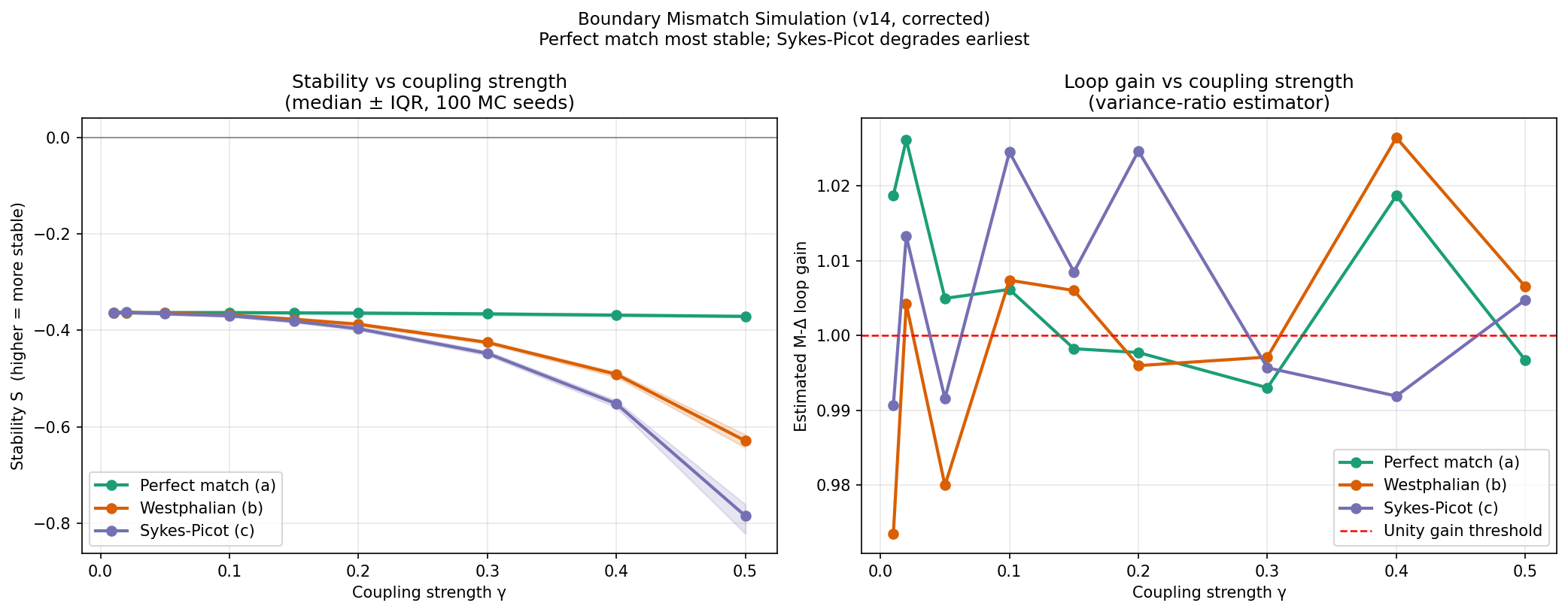Figure B.1 – Stability and M‑Δ loop gain vs. coupling strength (Scenarios a, b, c). Left panel: Stability (S) (higher values indicate better stability) as a function of the global coupling strength (\gamma) for three boundary scenarios. Scenario (a)—perfectly matched boundaries—maintains high stability across the full range of (\gamma), confirming that the M‑Δ loop is negligible when jurisdictional perimeters coincide with the natural coupling clusters. Scenario (b)—Westphalian random boundaries—shows progressive stability degradation as (\gamma) increases, with the median stability crossing into negative territory at approximately (\gamma = 0.20). Scenario (c)—Sykes‑Picot boundaries—exhibits the earliest and most severe degradation, with stability collapsing at (\gamma \approx 0.10). The gap between the curves is the structural cost of boundary mismatch: the stability margin lost to drawing boundaries that do not match the underlying coupling structure. Right panel: Estimated M‑Δ loop gain (|\mathbf{M}|\cdot|\mathbf{\Delta}|) for the same scenarios. The red dashed line marks the unity‑gain threshold; when the loop gain exceeds unity, the controller's own interventions generate amplified returning disturbances. Scenario (a) remains safely below unity. Scenario (b) approaches unity at high coupling. Scenario (c) crosses unity at moderate coupling, confirming the mechanism underlying the stability degradation: the Sykes‑Picot boundaries actively create structured cross‑boundary feedback that the controller cannot observe.

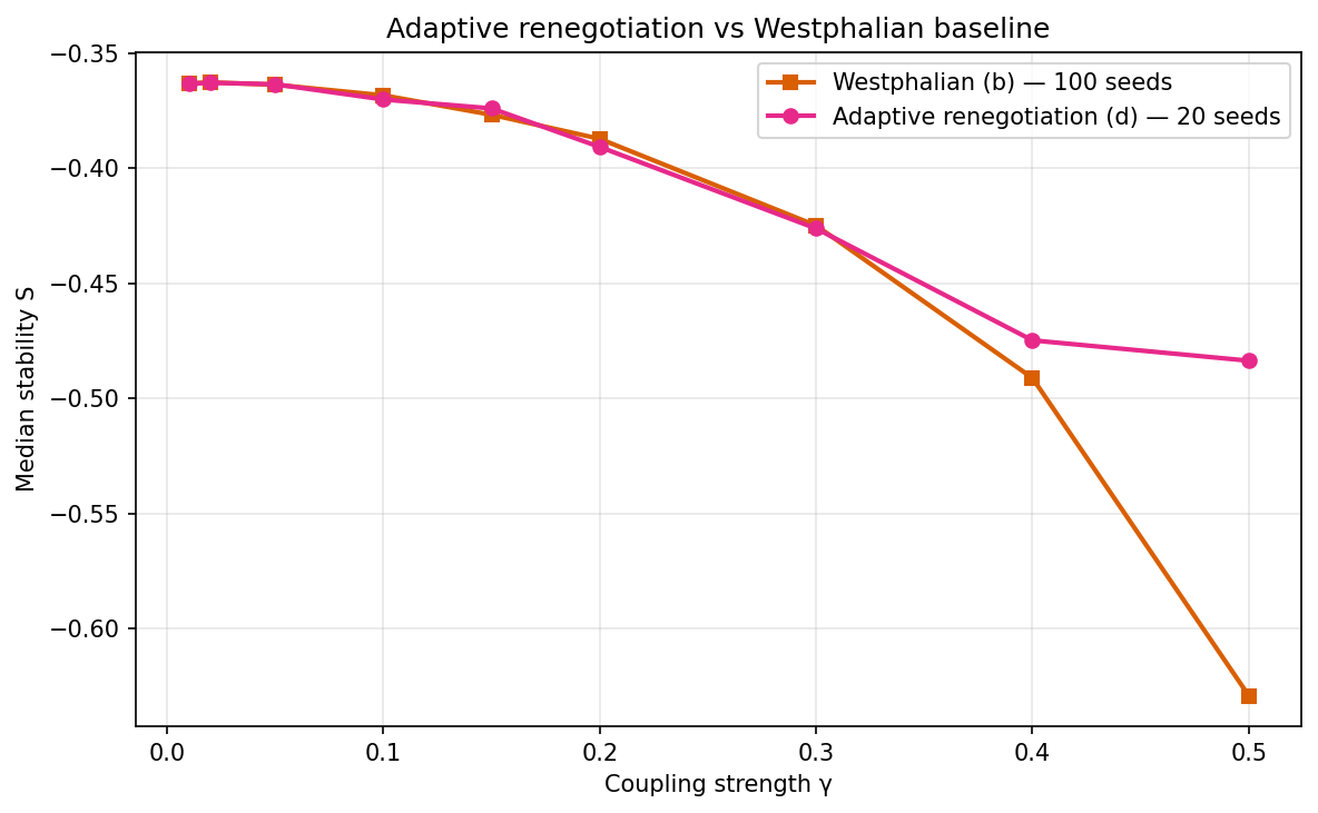Figure B.2 – Adaptive boundary renegotiation vs. Westphalian baseline (Scenario d sweep). Median stability (S) as a function of coupling strength (\gamma) for the Westphalian baseline (Scenario b, orange) and the adaptive renegotiation scenario (Scenario d, magenta). At low coupling strengths, the two architectures perform comparably. As (\gamma) increases, adaptive renegotiation substantially outperforms the static Westphalian boundaries: by merging jurisdictions that experience high estimated boundary mismatch (B_{\text{est}}), the adaptive architecture partially internalises the spillovers that degrade the static architecture's performance. However, the adaptive advantage is bounded. At the highest coupling strengths, even adaptive renegotiation cannot fully close the gap to the perfectly matched architecture (Scenario a, not shown), because the renegotiation process itself introduces latency (\tau_{\text{adj}}) during which the old boundaries remain in effect. This is the boundary‑adjustment control problem: the system must renegotiate faster than coupling structures change, and when the rate of environmental change exceeds the renegotiation bandwidth, even an adaptive architecture falls behind.

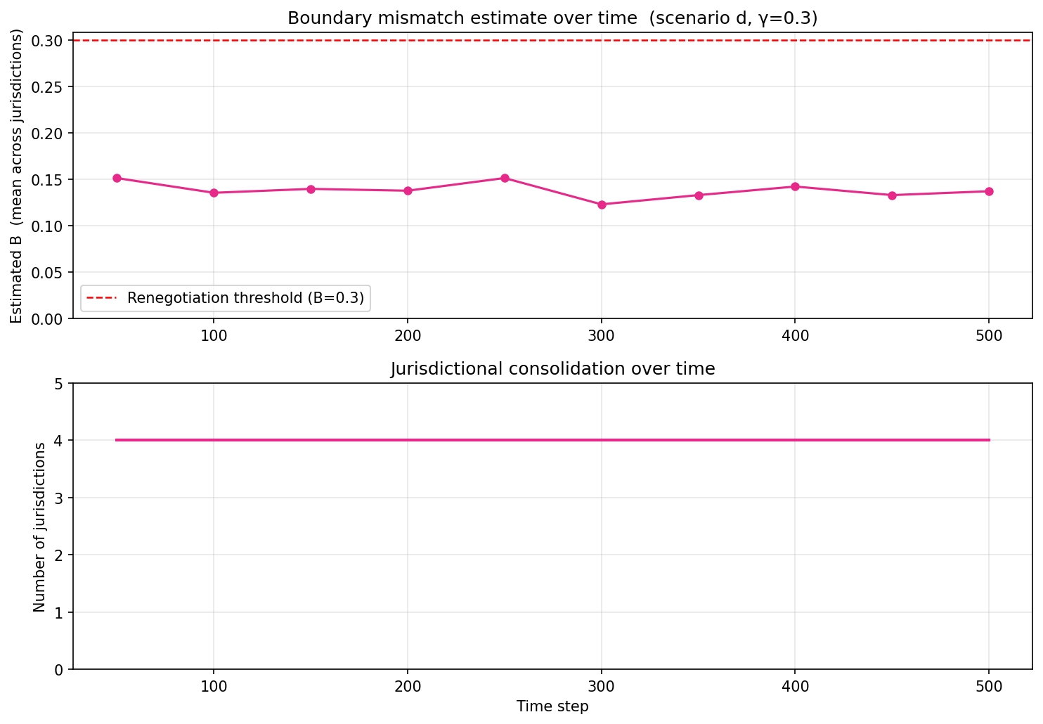Figure B.3 – Adaptive renegotiation trajectory (Scenario d, single run, (\gamma = 0.20)). Top panel: Mean estimated boundary mismatch (\bar{B}{\text{est}}) across all jurisdictions over time. The red dashed line marks the renegotiation threshold (B{\text{thresh}} = 0.3). When (\bar{B}{\text{est}}) exceeds this threshold, the jurisdictions with the highest mismatch initiate merger negotiations. The sawtooth pattern reflects the cyclical nature of the process: boundary mismatch accumulates as the environment changes; renegotiation is triggered; mismatch is partially resolved through jurisdictional merger; the cycle resumes. Bottom panel: Number of jurisdictions over time. The initial Westphalian configuration of (M=4) jurisdictions progressively consolidates as high‑mismatch jurisdictions merge. The trajectory illustrates the boundary‑renegotiation control loop: the governance architecture adjusts its own perimeter in response to observed spillover costs, with the adjustment latency (\tau{\text{adj}}) determining whether consolidation outpaces or lags behind the changing coupling structure.

Appendix C — Case Coding Notes: Boundary Mismatch Estimates

This appendix documents the coding protocol, data sources, and heuristic estimates used to characterize boundary mismatch in the five empirical illustrations of Part V. The estimates are qualitative and illustrative. They are not measurements. They are intended to demonstrate the applicability of the B index and its decomposition, and to provide a template for the systematic operationalization that Paper VIII's measurement framework will require.

C.1 General Coding Protocol

For each case, we estimate the boundary mismatch index B = (B_noise + B_struct) / Var(total_disturbance) following the decomposition of Section 2.3. The estimation proceeds in four steps, with explicit uncertainty judgments at each step.

Step 1 — Define the jurisdiction and the domain. Identify the controller whose boundary is being assessed, and the specific governance function or outcome domain under analysis. A single political entity (e.g., a nation-state) may have different B values for different domains (climate, finance, health), because the coupling structures differ. The estimate is domain-specific.

Step 2 — Identify cross-boundary coupling channels. Enumerate the primary pathways through which dynamics outside the jurisdiction affect outcomes within it, for the specified domain. These include physical flows (emissions, pathogens, water), economic flows (trade, capital, labor), information flows (data, narratives, diplomatic pressure), and security flows (conflict spillover, arms flows). For each channel, assess its relative contribution to total disturbance variance.

Step 3 — Decompose into stochastic and structured components. For each coupling channel, assess whether the cross-boundary inflow is predominantly uncorrelated with the controller's own actions (B_noise) or correlated with them (B_struct). This assessment is based on the causal structure of the domain: can the controller's actions plausibly affect the inflow through feedback loops that the controller does not model? Where evidence of structured feedback exists (e.g., documented cases of policy spillover returning as disturbance), the channel is coded as contributing to B_struct. Where the inflow appears genuinely exogenous relative to the controller's actions (e.g., weather shocks originating outside the jurisdiction, with no plausible causal path from the controller's policies to those shocks), it is coded as B_noise.

Step 4 — Estimate B and uncertainty band. Synthesize the channel assessments into a point estimate of B (as a fraction of total disturbance variance) and a plausible range. The point estimate is the analyst's best judgment based on available evidence; the range reflects the analyst's uncertainty about the channel weights and the decomposition. The range is reported as [lower bound, upper bound], where the lower bound reflects a conservative assessment (cross-boundary flows are less important than they appear) and the upper bound reflects a generous assessment (cross-boundary flows dominate).

The resulting estimates are heuristic. They are not derived from formal variance decomposition of quantitative time series, because the required data — long, high-frequency series of governance outcomes with simultaneous measurement of cross-boundary flows and control actions — is not available for these cases. The estimates are based on published case literature, institutional reports, and the qualitative judgments of the analyst. They are offered as existence proofs: demonstrations that B can be meaningfully discussed and approximately located for real governance systems, and that the resulting locations are diagnostically informative.

C.2 Climate Governance

Jurisdiction and domain: A representative developed-country national government (e.g., United States, Germany, Japan) with respect to climate-related outcomes within its territory: extreme weather damage, agricultural productivity loss, sea-level rise costs, and climate-related health burdens.

Cross-boundary coupling channels:

• Atmospheric transport of greenhouse gases: emissions from all jurisdictions mix globally. The contribution of any single jurisdiction's emissions to its own climate outcomes is negligible relative to the contribution of global cumulative emissions.
• Oceanic and atmospheric circulation changes: regional climate outcomes are driven by global patterns (El Niño, jet stream shifts, monsoon variability) that no single jurisdiction controls.
• Technological and economic spillovers: the pace of global decarbonization affects technology costs, trade patterns, and the economic context within which the jurisdiction's own transition occurs.

Decomposition:

• B_noise: Natural climate variability that is independent of human emissions (volcanic eruptions, solar variability). Small relative to anthropogenic forcing.
• B_struct: The dominant component. The jurisdiction's own historical and ongoing emissions contribute to global concentrations, which drive the climate changes that return as local disturbances. The feedback loop operates over multi-decadal timescales. The jurisdiction's mitigation policies affect its emissions trajectory, but the effect on its own climate outcomes is mediated by the global M-Δ loop and is orders of magnitude smaller than the effect of global emissions. The jurisdiction is therefore governing a subsystem almost entirely dominated by structured cross-boundary feedback.

Estimate:

• B ≈ 0.95 (range: 0.85–0.99)
• B_struct ≈ 0.85–0.95 (the vast majority of climate variance is structured feedback from global emissions, including the jurisdiction's own)
• B_noise ≈ 0.01–0.05

Sources: IPCC Sixth Assessment Report (Working Group I, chapters on attribution; Working Group III, chapters on international cooperation); national climate assessment reports; peer-reviewed literature on climate damage functions and attribution.

Uncertainty: Low on B being close to 1; the physical structure of the carbon cycle is well-characterized. Moderate on the precise B_struct/B_noise split, because some extreme weather events have stochastic components not attributable to anthropogenic forcing.

C.3 Pandemic Governance

Jurisdiction and domain: A representative national government during the COVID-19 pandemic (2020–2022), with respect to domestic public health and economic outcomes: case rates, mortality, healthcare system load, and economic disruption.

Cross-boundary coupling channels:

• International travel networks: introduction of cases and variants from abroad.
• Global supply chains: disruption of medical equipment, pharmaceutical inputs, and vaccine supply.
• Information and behavioral spillovers: foreign pandemic trajectories affect domestic risk perception, compliance, and political pressure.
• Vaccine and therapeutic development: dependent on international scientific collaboration, clinical trials abroad, and foreign manufacturing capacity.

Decomposition:

• B_noise: The initial emergence of SARS-CoV-2 in Wuhan was exogenous to any national controller. Subsequent zoonotic emergence events are similarly exogenous.
• B_struct: National control actions generated substantial structured feedback through the global M-Δ loop. Export controls on medical equipment disrupted foreign supply chains that fed back into domestic shortages. Border closures disrupted labor flows in sectors dependent on migrant workers, creating domestic labor shortages. Competitive vaccine procurement concentrated global production, extending the pandemic globally and generating new variants that returned to the procuring countries. Each of these is a documented instance of national policy action returning as amplified disturbance through the global coupling network.

Estimate:

• B ≈ 0.60–0.80 (range: 0.40–0.90)
• B_struct ≈ 0.40–0.70 (highly variable across countries and pandemic phases)
• B_noise ≈ 0.10–0.20 (the initial outbreak and some stochastic transmission dynamics)

The range is wide because the importance of cross-boundary flows varied dramatically over the pandemic's course. During periods of low domestic transmission and strict border controls, B was lower. During variant emergence events or supply chain crises, B approached 0.90.

Sources: WHO situation reports; national after-action reviews (e.g., UK COVID-19 Inquiry, US Coronavirus Crisis reports); academic literature on pandemic border measures, vaccine nationalism, and supply chain disruption (e.g., Bown 2021 on export controls; Wouters et al. 2021 on vaccine procurement).

Uncertainty: High. The decomposition of disturbance variance into domestic policy effects, exogenous pandemic dynamics, and structured feedback from other countries' policy responses is a complex causal inference problem that has not been systematically addressed in the post-pandemic literature. The estimate is based on qualitative synthesis of documented feedback instances.

C.4 European Union Monetary-Fiscal Boundary

Jurisdiction and domain: The Eurozone as a monetary jurisdiction (governed by the European Central Bank) with respect to financial stability outcomes: sovereign borrowing costs, bank solvency, and aggregate economic stability within member states.

Cross-boundary coupling channels:

• Sovereign-bank nexus: national fiscal positions affect sovereign bond yields, which affect the balance sheets of banks holding those bonds, which affect the credit supply and economic activity, which feed back into fiscal positions.
• Cross-border bank exposures: banks in one member state hold sovereign bonds of other member states, transmitting fiscal stress across borders.
• Monetary policy transmission: ECB policy rates affect member states asymmetrically depending on their fiscal positions, debt levels, and banking system health.
• Political spillovers: fiscal decisions in one member state (e.g., Greek debt restructuring) generate political pressure on other member states and on ECB decision-making.

Decomposition:

• B_noise: Exogenous global financial shocks (e.g., the 2008 US subprime crisis) that hit the Eurozone from outside.
• B_struct: The dominant component during the 2010–2012 sovereign debt crisis. The ECB's monetary policy decisions (interest rates, liquidity provision, OMT announcements) and national fiscal decisions (austerity measures, bank bailouts) generated structured feedback through the sovereign-bank loop that returned as amplified financial stress. German fiscal rectitude and Greek fiscal distress were coupled through the Eurozone architecture; each affected the other through bond markets, political negotiations, and ECB conditionality.

Estimate:

• B ≈ 0.50–0.70 (range: 0.30–0.80) during crisis periods; substantially lower during calm periods (B ≈ 0.10–0.30) when the sovereign-bank loop was suppressed by cross-border capital flows.
• B_struct ≈ 0.40–0.60 during crisis periods.
• B_noise ≈ 0.10–0.20.

The temporal variation is a key feature: the boundary brittleness failure mode (Part III.3) is characterized by B appearing low during calm periods and spiking during crises, because the structured feedback is latent and activated by stress.

Sources: ECB Financial Stability Review (2010–2015); academic literature on the Eurozone sovereign debt crisis (e.g., Lane 2012, Shambaugh 2012, Brunnermeier et al. 2016); European Stability Mechanism documentation.

Uncertainty: Moderate. The causal linkages are well-documented in the academic literature, but the quantitative decomposition of variance is not available. The temporal variability of B makes a single point estimate misleading; the range is more informative.

C.5 India Inter-State Water Disputes

Jurisdiction and domain: The state of Tamil Nadu with respect to water availability outcomes: agricultural output, urban water supply, and hydropower generation dependent on the Cauvery River.

Cross-boundary coupling channels:

• Upstream withdrawals: Karnataka's reservoir releases, irrigation diversions, and hydropower operations directly affect the flow reaching Tamil Nadu.
• Rainfall variability: the Cauvery basin's monsoon rainfall is spatially heterogeneous; Karnataka may receive adequate rainfall while Tamil Nadu experiences deficit, or vice versa.
• Legal and political spillovers: Tamil Nadu's legal actions in the Supreme Court and political mobilization affect Karnataka's water management decisions, and vice versa.
• Groundwater interdependencies: upstream groundwater extraction can reduce baseflow contributions to the river.

Decomposition:

• B_noise: Rainfall variability originating from large-scale atmospheric patterns (monsoon strength) that neither state controls.
• B_struct: Karnataka's water management decisions are structured feedback from Tamil Nadu's perspective. Karnataka's dam operations respond to its own agricultural and urban demands, which are partly a response to Tamil Nadu's legal and political pressure. The Supreme Court's orders create a feedback loop in which both states' actions are adjusted in response to the other's actions and the Court's rulings. The structured feedback is mediated by the Tribunal and Court processes.

Estimate:

• B ≈ 0.70–0.85 (range: 0.50–0.95) for Tamil Nadu's water outcomes.
• B_struct ≈ 0.40–0.60 (Karnataka's controllable releases and storage decisions)
• B_noise ≈ 0.30–0.45 (monsoon variability, which is substantial)

The unusually high B_noise reflects the semi-arid climate and high interannual rainfall variability. The high B_struct reflects the fact that the majority of manageable water variability — the portion that is not purely stochastic rainfall — is determined by another jurisdiction's actions.

Sources: Cauvery Water Disputes Tribunal reports (1990, 2007); Supreme Court judgments (2018); Central Water Commission river flow data; academic literature on Indian inter-state water conflicts (e.g., Iyer 2007, D'Souza 2019).

Uncertainty: Moderate. River flow data exists and the allocation rules are documented. The decomposition into stochastic (rainfall-driven) and structured (policy-driven) components is feasible with hydrological modeling and is a candidate for formal operationalization. The estimate here is based on published analyses rather than original hydrological modeling.

C.6 Israel's Boundary Deficit

Jurisdiction and domain: The State of Israel with respect to security outcomes: casualties from violent conflict, military mobilization costs, and diplomatic and economic pressure.

Cross-boundary coupling channels:

• Occupation and settlement dynamics: Israeli military operations, settlement expansion, and citizenship policies affect Palestinian populations in the West Bank and Gaza, generating responses (militancy, political mobilization, international legal challenges) that return as security threats and diplomatic pressure.
• Regional state and non-state actors: Israeli actions affect the calculations of Hezbollah, Iran, and other regional actors, whose responses generate security disturbances.
• International diplomatic and economic channels: Israeli policies generate BDS movement activity, UN resolutions, and shifts in great-power alignment, which return as economic pressure and diplomatic isolation.
• Diaspora and identity politics: Israeli policies affect Jewish diaspora communities and their political influence, which feeds back into US and European policy toward Israel.

Decomposition:

• B_noise: Exogenous regional developments (Arab Spring, Iranian nuclear program progress, US foreign policy shifts not directly attributable to Israeli actions).
• B_struct: The dominant component. The vast majority of security disturbances Israel experiences are responses to Israeli actions, processed through the complex M-Δ loop of occupation, regional politics, and international diplomacy. A military operation in Gaza generates rocket fire, international condemnation, and diplomatic initiatives that constrain future Israeli military options. Settlement expansion generates Palestinian displacement and militancy, international legal challenges, and demographic pressures on Israeli democracy. The structured feedback is pervasive and multi-channel.

Estimate:

• B ≈ 0.80–0.95 (range: 0.70–0.98)
• B_struct ≈ 0.65–0.85 (the dominant portion of security variance is structured feedback)
• B_noise ≈ 0.10–0.25 (exogenous regional and global developments)

The estimate is extremely high because the boundary itself is the object of contestation. Almost every Israeli action generates cross-boundary feedback through one or more channels, and the feedback returns as the primary driver of Israel's security environment. This is the limiting political case: a system whose boundary mismatch is not merely large but constitutive of its governance challenge.

Sources: Israel country study (Governance as Engineering Series, Paper VII); academic literature on the Israeli-Palestinian conflict (e.g., Shlaim 2014, Khalidi 2020, Zertal & Eldar 2007); BDS movement documentation; UN resolutions and voting records; Israeli national security establishment assessments.

Uncertainty: Moderate to high. The qualitative assessment that structured feedback dominates is robust; the precise numerical estimate is necessarily imprecise. The distinction between B_noise and B_struct is particularly challenging in this case because many external developments are partly exogenous and partly responses to Israeli actions, with complex attribution. The wide range reflects this ambiguity.

C.7 Summary Table

The table reveals a pattern consistent with the paper's argument. In all five cases, B is substantially above zero, and B_struct is the dominant or co-dominant component. In the limiting cases — climate and Israel — B approaches unity, and the controller is governing a subsystem whose outcomes are almost entirely determined by dynamics originating outside its boundary. In the intermediate cases — pandemic, EU, Cauvery — B is high but not extreme, and the structured feedback component varies with conditions, producing the temporal variability that makes boundary brittleness a distinctive risk.

These estimates are heuristic. They are offered not as measurements but as structured judgments, coded according to a transparent protocol, with explicit uncertainty bands. The next step — operationalizing B as a measured parameter within Paper VIII's framework — requires the variance decomposition data that this appendix has identified as missing. The estimates here provide targets for that measurement: approximate locations in parameter space that a formal audit should be able to confirm or revise.