This paper follows Papers XVI and XVII in the limits-of-perception cluster and returns their results to an engineering register. Paper XII established that a wrongly drawn jurisdictional boundary destabilizes an otherwise competent controller; its adaptive scenario showed boundaries chasing an externally shifting coupling landscape. This paper treats the case Paper XII's formalism excluded by construction: coupling that shifts because the controller learns. All formal results are tagged [R within the model] and proven or exhibited in Appendix A; the institutional readings are [IP]; the confidence discipline of the series applies throughout, and §9 states what the paper does not show.

Abstract

Paper XII modeled the gap between a controller's jurisdiction and the world as an M–Δ feedback interconnection and showed that a mismatched boundary can destabilize a system every component of which is internally sound. That analysis held the coupling structure exogenous: the boundary is a container, and the question is whether it is drawn correctly. This paper removes the exogeneity assumption. When a governance system's learning acts through channels that also carry cross-boundary influence — when $\partial \mathbf{\Delta }/\partial \theta \ne 0$ — the decomposition into "jurisdiction" and "environment" becomes reflexive: coupling is policy-dependent, and factorizability is a property of the learning trajectory, not of the architecture.

We formalize factorizability as the existence of a common invariant-subspace pair of the parameterized matrix family $\{\mathbf{A}(\theta (t))\}$ and prove the Non-Factorizability Theorem [R within the model]: under generic persistent learning, the parameter trajectory escapes the compatibility variety of every fixed decomposition — the boundary that was correct at design time does not stay correct, and the process that un-corrects it is the controller's own adaptation. A minimal two-subsystem model exhibits the consequence as a reflexive boundary cycle: factorizable calm, hidden coupling accumulation, non-factorizable collapse, miscalibrated recovery. Simulation establishes the cycle in a non-degenerate parameter region, bounded above by a regime the outline did not anticipate — a locked non-factorizable state from which the boundary never recovers.

Two further results follow. First, a Critical Learning Bandwidth ${\eta }_{\min }(r_{\text{env}})\le \eta \le {\eta }_{\max }(\partial \mathbf{\Delta }/\partial \theta )$: learning too slow loses the plant (Paper XV's bound, in local form), learning too fast dissolves the boundary through the policy-velocity coupling channel, and the two bounds pinch endogenously — the window closes on a substantial region of parameter space, a zero-viability condition we call the Decomposability Frontier. Second, a negative result the registered predictions forced us to keep: the Boundary Dissolution Index defined on cross-boundary prediction-error covariances fails as an early-warning signal, because local adaptation absorbs coupling into gain and thereby launders the evidence out of exactly the residuals the index monitors — Goodhart's law applied to the diagnostic itself. The coupling remains visible in cross-boundary state covariances, and even there detection is lead-limited. Design principles follow for boundary-health monitoring, oscillation damping under a friction–timescale constraint, polycentric decomposability reserves, and external certification anchors, the last operationalizing Paper XVII's certification floor at its own confidence tier. The central governance challenge is reframed: not choosing the right boundary, but maintaining a decomposability margin under the boundary drift that learning inevitably induces.

1. Introduction: from fixed boundaries to reflexive decompositions

1.1 What Paper XII established, and what it held fixed

Paper XII gave the series its boundary primitive. A controller governs a modeled plant; the real plant is larger; the difference — the cross-boundary dynamics the controller's jurisdiction excludes — is the Δ block of an M–Δ feedback interconnection, and the small-gain theorem supplies the stability condition. When the loop gain around the unmodeled dynamics exceeds unity, the controller's own stabilization efforts return, processed through the external loop, as amplified disturbances. Three failure modes followed (spillover oscillation, cascading boundary failure, boundary brittleness), a boundary mismatch index B was defined, and the pooling paradox established that no single-boundary architecture escapes the Information–Actuation Frontier: expanding the boundary internalizes coupling at the cost of chain length; shrinking it preserves fidelity at the cost of ungoverned feedback.

Paper XII also went one step further than a static analysis, and it matters for locating this paper precisely. Its Scenario (d) allowed adaptive boundary renegotiation: jurisdictions adjusting their perimeters as coupling patterns shift. The finding was that renegotiation introduces its own M–Δ lag loop, and fails beyond a critical rate of environmental change relative to renegotiation capacity. But throughout — in the static scenarios and the adaptive one alike — the coupling structure itself was exogenous. Boundaries chase a landscape that shifts for reasons of its own: technological change, economic integration, environmental drift. The controller's learning adjusts to the coupling; it does not create it.

1.2 The reflexivity gap

That exogeneity assumption fails for the systems governance cares most about, and it fails structurally rather than incidentally. A regulator that tightens capital requirements changes the routing of financial flows across its perimeter. A jurisdiction that learns to tax a mobile base teaches the base to move, creating cross-border arbitrage channels that did not previously carry weight. A platform that adapts its moderation policy reshapes which communities straddle its boundary with the open web. In each case the policy parameters $\theta$ that the controller adjusts are also arguments of the coupling: $\partial \mathbf{\Delta }/\partial \theta \ne 0$. The controller's learning does not merely respond to the boundary's adequacy — it is one of the forces determining it.

This is the gap the present paper fills, and the claim is deliberately stronger than "boundaries need maintenance." The claim is that under generic learning, no fixed decomposition of the world into jurisdiction and environment remains exact along the trajectory — the boundary that was correct when drawn is un-corrected by the very adaptation it encloses (§2) — and that the resulting dynamics have a characteristic shape: a cycle of factorizable calm, hidden accumulation, collapse, and miscalibrated recovery (§3), governed by a learning-rate window that can close entirely (§4).

1.3 The adaptive-control precedent

The core phenomenon has a rigorously established ancestor, and citing it locates the paper's contribution honestly. Rohrs and colleagues showed in 1985 that adaptive controllers satisfying every then-standard convergence condition could be destabilized by unmodeled dynamics — precisely because persistent adaptation keeps exciting the plant through channels the reference model omits, and the adaptation law, reading the resulting error as parameter mismatch, chases it. The subsequent averaging literature derived the repair as a slow-adaptation condition: the adaptation rate must remain below a bound set by the unmodeled dynamics' time constants. The structural insight — that adaptation and unmodeled coupling form a destabilizing pair, with a speed limit as the resolution — is established at [R] in that literature. What this paper does is transpose the structure to jurisdictional boundaries, where the "unmodeled dynamics" are the cross-boundary couplings a governance architecture excludes by design, and where the transposition adds an element the control-theoretic setting lacks: the boundary itself is an institutional variable, with its own dynamics of clarity, collapse, and recovery. The transposition is [IP]; the model results built on it are [R within the model]; nothing in this paper strengthens or weakens the adaptive-control results it borrows.

1.4 Scope condition: the reflexivity asymmetry

The framework applies to world-coupled coordination — governance, markets, ecologies — where coupling channels are influenced by behavior and the external world pushes back in ways not fully internalizable. It does not apply with the same force to purely self-referential systems, and the reason is worth stating carefully because it is an argument, not a corollary of the theorem. Nothing in the mathematics of §2 prevents its hypotheses from holding inside a closed symbolic game. The asymmetry lies elsewhere: a self-referential system may redefine its decomposition by convention as the trajectory moves — when the facts on both sides of a boundary are conventions, re-factorization is free — whereas a world-coupled system must compensate drift it cannot rename. The theorem says every fixed decomposition is escaped; the domains differ in the price of re-fixing. This mirrors, and is disciplined by, the world-coupled/self-referential scope bound of Paper XVII.

1.5 Plan

Section 2 states the Non-Factorizability Theorem, with proof in Appendix A.1. Section 3 specifies the minimal reflexive model, reports the simulated boundary cycle, and reports the falsification of one registered prediction. Section 4 derives the Critical Learning Bandwidth and exhibits its closure. Section 5 revises the Boundary Dissolution Index in light of §3's negative result. Section 6 derives design principles. Section 7 integrates with the series; Section 8 concludes; Section 9 records what the paper does not show.

2. The Non-Factorizability Theorem

2.1 Factorizability is an invariant-subspace condition

The formal object must be chosen with care, because the natural first formalization proves the wrong thing. It is not the case that a fixed decomposition requires the coupling block $\mathbf{\Delta }$ to be constant; a coupling that varies in magnitude while respecting a fixed zero pattern is factorizable forever, and a "theorem" concluding only that $\mathbf{\Delta }(\theta (t))$ is time-varying would restate its own hypothesis. What a fixed decomposition requires is that some single projection $\mathbf{\Pi }$ — some one way of splitting the state space into jurisdiction $\mathcal{S}$ and environment ${\mathcal{S}}^{\perp }$ — keeps both cross-influence blocks at zero for every parameter value the learning trajectory visits:

$$\mathbf{\Pi }\mathbf{A}(\theta (t))(\mathbf{I}-\mathbf{\Pi })=0,(\mathbf{I}-\mathbf{\Pi })\mathbf{A}(\theta (t))\mathbf{\Pi }=0\text{for all }t.$$

Equivalently: $\mathcal{S}$ and ${\mathcal{S}}^{\perp }$ are a common invariant-subspace pair of the matrix family $\{\mathbf{A}(\theta (t)){\}}_t$. For a fixed $\mathbf{\Pi }$, the parameter values compatible with it form the compatibility variety ${\mathcal{V}}_{\mathbf{\Pi }}\subset \Theta$ — the zero set of the $2d(n-d)$ off-diagonal entries as functions of $\theta$. Factorizability along a trajectory is confinement to ${\mathcal{V}}_{\mathbf{\Pi }}$; boundary drift is escape from it. This reformulation is what makes the theorem non-trivial: common invariant subspaces of matrix families are a genuinely restrictive condition, and whether a learning trajectory respects one is a question about the geometry of the learning field relative to the variety, not about whether anything varies.

2.2 Statement

Theorem (Non-Factorizability, [R within the model]; Appendix A.1). Fix any split $\mathbf{\Pi }$ and suppose: (i) non-degeneracy — the coupling sensitivity $\partial \mathbf{\Delta }/\partial \theta$ has rank at least one along the visited portion of ${\mathcal{V}}_{\mathbf{\Pi }}$, so the variety has positive codimension in $\Theta$; (ii) transversality — the averaged learning field is not tangent to ${\mathcal{V}}_{\mathbf{\Pi }}$ on any open piece of it; (iii) persistence — the trajectory does not converge to a stationary point inside ${\mathcal{V}}_{\mathbf{\Pi }}$. Then the parameter trajectory leaves ${\mathcal{V}}_{\mathbf{\Pi }}$ in finite time. Since the argument applies to every admissible $\mathbf{\Pi }$, no time-invariant system–environment decomposition survives learning: factorizability is a transient, trajectory-dependent property, not a structural invariant.

Under stochastic learning — noise entering the update with an absolutely continuous distribution, as in this paper's own simulation — escape is almost sure by a measure argument alone, since ${\mathcal{V}}_{\mathbf{\Pi }}$ has measure zero under (i). The deterministic and stochastic statements rest on different hypotheses (transversality versus absolute continuity) and are kept separate; the paper never writes "almost surely" of a deterministic flow.

The proof (A.1.2) is short once the object is right: confinement to the variety would force the learning increments into its tangent bundle along a non-trivial visited set, which (ii) — or, stochastically, the measure-zero property — denies.

2.3 What the theorem does and does not license

Three restraints, each load-bearing for the rest of the paper.

The theorem is conditional on transversality, and that condition is a design surface. A learning rule engineered to act only through block-respecting channels — its field lying in the tangent bundle of ${\mathcal{V}}_{\mathbf{\Pi }}$ by construction — preserves factorizability indefinitely. The theorem's content is that this alignment is a codimension condition rather than a default: generic learning that reaches any coupling-relevant channel breaks every fixed split. Read forward, this is the formal seed of §6: the design principles are attempts to engineer the failure of hypothesis (ii) — to confine institutional learning, or at least its fastest components, to boundary-respecting directions.

Escape is qualitative; damage is quantitative. Leaving ${\mathcal{V}}_{\mathbf{\Pi }}$ means the decomposition ceases to be exact. How fast the off-diagonal blocks then grow, and whether the M–Δ loop gain of Paper XII crosses unity, the theorem does not say; that is the work of §§3–4. A system may live arbitrarily long with a slightly inexact boundary. The theorem forbids only the comfortable belief that a correct boundary, once drawn, is a settled matter.

The corollaries inherit the tier, not more. Corollary 1 (spectral drift, [R within the model]): any stability certificate evaluated at $\theta (0)$ — including Paper XII's small-gain condition — is not invariant under learning satisfying (i)–(iii); stability is a property of the joint plant–controller–learning trajectory. Corollary 2 (environment as field, [R within the model]): along such a trajectory $\mathbf{\Delta }(\theta (t))$ is a policy-dependent interaction field, and treating it as an exogenous operator mis-specifies the stability problem from the first step. The regress result — that hierarchies of meta-adaptive layers reproduce the drift at every level unless terminated by a $\theta$-independent anchor — is stated and proven within the model in Appendix A.4 and taken up in §6.4, where its relation to Paper XVII's [IP]-tier certification floor is drawn with both tiers intact.

2.4 Reading the theorem institutionally

The institutional reading, at [IP]: a constitution's allocation of competences, a federation's division of powers, a regulatory perimeter, an inter-agency memorandum of understanding — each is a choice of $\mathbf{\Pi }$, and each was, at best, an element of ${\mathcal{V}}_{\mathbf{\Pi }}$ at the moment of drafting: a parameter configuration under which the allocated domains genuinely did not couple. The theorem's translation is that the drafting moment does not propagate. Institutions that learn — that adjust tax schedules, capital rules, procurement practices, enforcement priorities — move $\theta$ through the ambient space, and the configurations compatible with the drafted boundary are a measure-zero subset of it. The familiar complaint that a constitutional division of powers "no longer fits" the coupled reality of finance, information, or climate is, in this frame, not evidence that the drafters chose badly. It is the expected fate of any fixed $\mathbf{\Pi }$ under a century of parameter motion, most of it induced by the governed system's own adaptation. The design question this poses — since redrawing $\mathbf{\Pi }$ is costly in exactly the ways Paper XII's pooling paradox and transition-bandwidth constraints describe — is not how to find the drift-proof boundary, which does not exist, but how to manage the margin. That question is taken up from §4 onward.

3. The reflexive boundary cycle: a minimal model

3.1 Specification

The model instantiates the theorem's hypotheses in the smallest system that can exhibit their consequences: two scalar subsystems, each governed by a local controller that believes its jurisdiction is closed and its model calibrated, coupled through a channel whose strength depends on both the states and the institutional variables. The full specification, with parameter values, is in the simulator header (paper_xviii_boundary_instability.py); the structure is:

$$x_i(t+1)=(a_t-k_i)x_i+\epsilon (t)x_j+w_i,\epsilon ={\epsilon }_0+\alpha (1-b)+\beta c,$$

$$c(t+1)=(1-\mu )c+\mu x_1{x}_2+\nu (|\Delta k_1|+|\Delta k_2|),b(t+1)=\sigma (\gamma (1-\overline{|r|}/R)-\delta |\epsilon |+h(b-\frac{1}{2})).$$

Each subsystem predicts its next state from its own closed model, ${\hat{x}}_i=(a_0-k_i)x_i$, so the residual $r_i=x_i(t+1)-{\hat{x}}_i=(a_t-a_0)x_i+\epsilon x_j+w_i$ is exactly the unmodeled content: drift staleness plus cross-boundary influence plus noise. Learning is a gradient step on the local squared residual with a leak, $k_i\leftarrow (1-\lambda )k_i+\eta x_i{r}_i$; states are soft-saturated at a finite range.

Five modeling choices are declared rather than hidden, because each is load-bearing and each was forced by an identifiable failure of the naive specification. The gain leak $\lambda$: without it the gain update is a ratchet and no relaxation oscillation is possible; institutionally, control effort is costly and un-renewed authority relaxes. The coupling stock $c$: the outline's instantaneous product $\beta x_1{x}_2$ cannot persist after a collapse, yet the outline's own phase narrative requires persistent coupling; the stock — coupling built by repeated interaction, decaying slowly — is the minimal persistence mechanism and the institutionally faithful one. The policy-velocity channel $\nu$: exploratory runs showed that with state-mediated reflexivity alone, faster learning is monotonically stabilizing and no upper learning-rate bound exists; the paper's premise $\partial \mathbf{\Delta }/\partial \theta \ne 0$ requires a direct channel, and $\nu$ — each side's rule changes create interfaces that entangle the jurisdictions — is its minimal implementation and the quantity §4 sweeps. The memory term $h(b-\frac{1}{2})$ is AR(1) self-excitation, not hysteresis proper; the earlier label is corrected. The closed-model residual replaces the outline's open-loop baseline: it makes $r_i$ the literal boundary-mismatch signal, at the price of one consequence recorded in §5. All five are in the simulator's changelog with the exploratory runs that forced them.

The correspondence to §2 is exact where it needs to be: $\theta =(k_1,k_2)$ reaches $\mathbf{\Delta }$ both indirectly through the states and directly through $\nu$, so hypothesis (i) holds by construction; the process noise makes escape a measure statement; and the "boundary" whose fate the theorem predicts appears twice, as the actual coupling $\epsilon$ and as the perceived clarity $b$ — the gap between the two is where the cycle lives.

3.2 The four phases, as exhibited

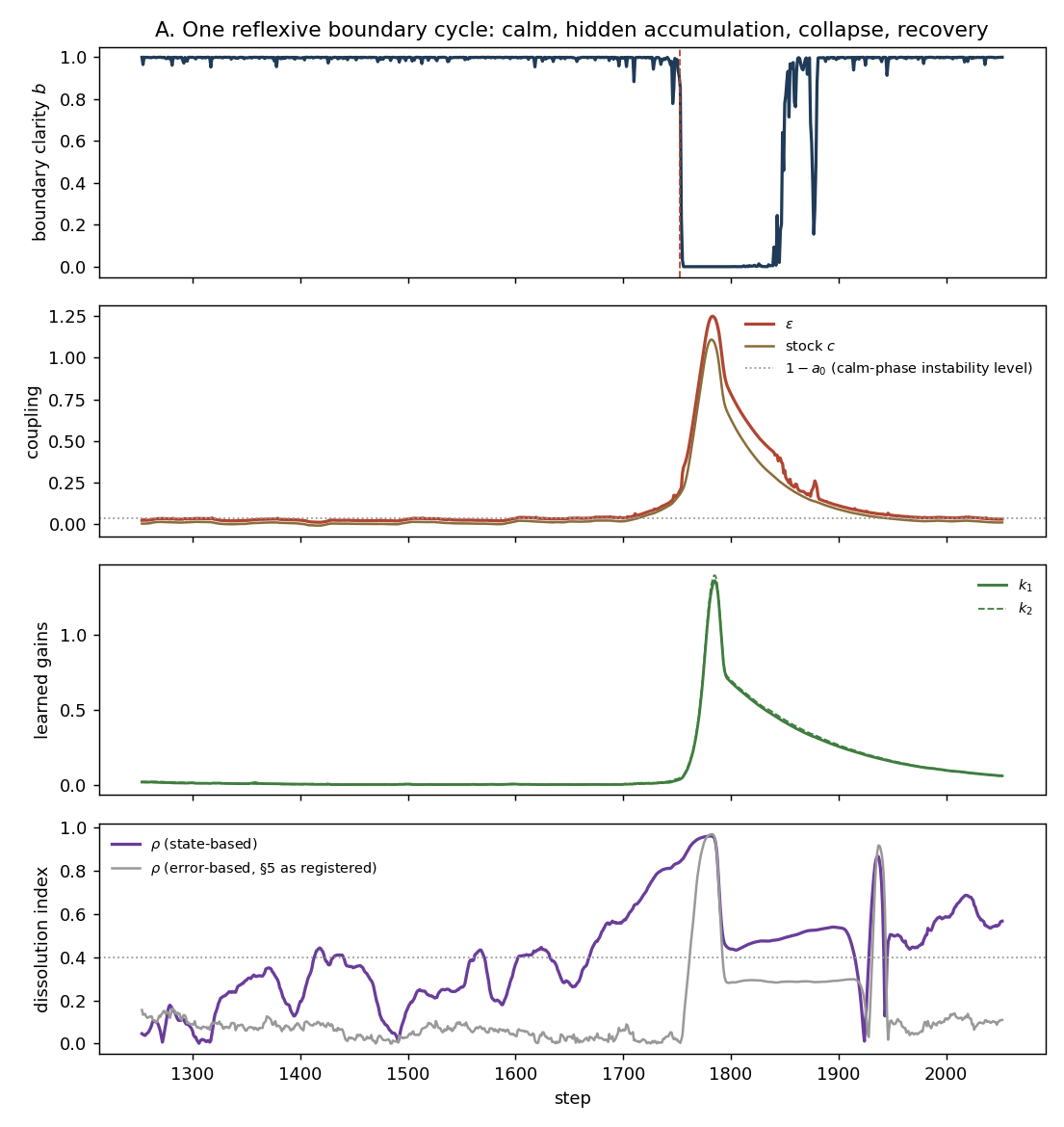
The simulated system (Figure xviii_A_phase_cycle) traverses the cycle the outline predicted, with one correction noted below. [R within the model] for the exhibited dynamics; the institutional glosses are [IP].

Factorizable calm. Boundary clarity high, coupling near its structural floor, gains near zero, local prediction good. Every internal indicator reports health, and the reports are, locally, true.

Hidden coupling accumulation. The interaction stock ramps: correlated states feed $c$, $c$ feeds $\epsilon$, $\epsilon$ correlates the states further. The compounding is invisible where the institutions are looking — residual magnitudes grow only with ${\epsilon }^2$ while the feedback compounds — and $b$ stays high because prediction error stays small. The closed-form fast statistics (A.2.2) locate the cliff this ramp approaches: the interaction statistic diverges as $\epsilon \to 1-(a-k)$, the margin the local gains leave open.

Non-factorizable collapse. The divergence is reached; states and coupling run away on the fast timescale until saturation bounds the excursion; residuals explode; each controller finds its local model invalid and its own actions returning as unattributable feedback; $b$ falls to its dissolved branch. The now-enormous learning signal drives the gains up fast — the panicked overcorrection is gain adaptation, not boundary redrawing.

Miscalibrated recovery. High gains kill the states; the residuals quiet; $b$'s clarity recovers because the symptoms have been suppressed — but the stock decays only slowly, so the system re-enters calm with real coupling still elevated and, as the leak bleeds the gains back down, the instability re-arms. The recovery is miscalibrated in exactly the sense the outline claimed, and the mechanism is now explicit: perceived clarity tracks residuals, residuals track what adaptation has absorbed, and adaptation has absorbed the evidence.

(Figure: xviii_A_phase_cycle.png — one cycle: the stock ramp under a quiet b, the ε excursion past 1−a₀, the gain spike, collapse and staggered recovery.)

3.3 Simulation results: the cycle exists, and it has a terminus (P1)

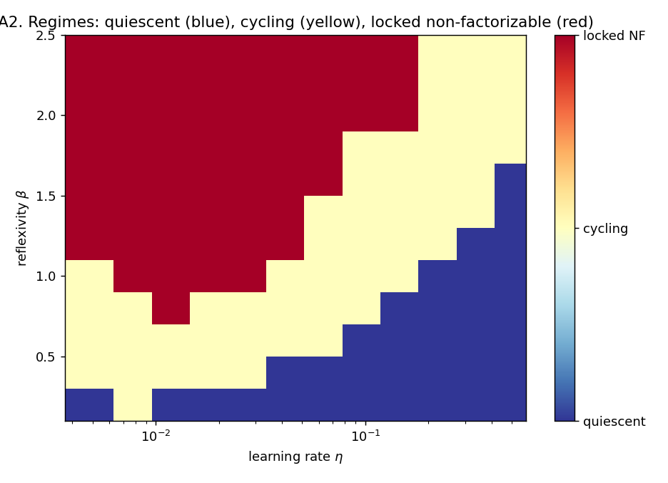
The registered prediction P1 — a sustained oscillation in a non-degenerate region of $(\beta ,\eta )$ space — is supported. The exhibit run produces nine collapse–recovery events in 6000 steps; the regime map (Figure xviii_A2_regime_map, a $12\times 12$ grid over $\beta \in [0.2,2.4]$, $\eta \in [0.005,0.5]$) classifies 36% of the grid as cycling. [R within the model.]

The map also contains a finding the outline did not anticipate, and it belongs in the phase narrative rather than in a footnote. The cycling region is bounded on one side by a quiescent regime — reflexivity too weak to reach the fold — and on the other by a locked non-factorizable regime: at high reflexivity, the post-collapse coupling floor ${\epsilon }_0+\alpha (1-b)$ is itself high enough to hold clarity at zero permanently. The boundary never recovers; the system settles into permanent NF residence. The cycle, in other words, is not the worst case. It is the intermediate case, available only to systems whose reflexivity is strong enough to break the boundary but weak enough that breaking it does not weld it shut. Institutionally [IP]: the oscillating pattern of crisis and reform presupposes a reflexivity regime; past it lies not faster oscillation but a permanently dissolved separation in which "jurisdiction" survives as a legal fiction over a fully coupled plant. Appendix A.2.3 gives the averaged planar reduction that explains the cycle's anatomy and states plainly why no analytic limit-cycle theorem is claimed for it.

(Figure: xviii_A2_regime_map.png — quiescent, cycling, and locked non-factorizable regimes over (β, η).)

4. The Critical Learning Bandwidth

4.1 Two bounds of different kinds

The cycle of §3 ran at a fixed environment. Add the series' standing pressure — an environment that drifts at rate $r_{\text{env}}$, here as $a_t=a_0+r_{\text{env}}t$ with the local models' calibration going stale — and the learning rate $\eta$ acquires two bounds whose mechanisms differ, not merely their directions.

The lower bound is Paper XV's, in local form. Learning must outrun staleness. The averaged gain flow (A.3.1) gives

$${\eta }_{\min }(t)\approx \frac{r_{\text{env}}+\lambda (a_t-a_0)}{{\sigma }_x^{2}m},$$

with $m$ the stability margin. The drift rate enters as expected. The leak term does something less expected and worth naming: ${\eta }_{\min }$ grows with the accumulated drift $(a_t-a_0)$ even at constant $r_{\text{env}}$ — where adaptive capacity decays (Paper XVI's territory), merely holding an already-absorbed adaptation costs standing learning rate. A system can fall below its own ${\eta }_{\min }$ without the world speeding up at all. [R within the model], averaged; unregistered but derived, and flagged as such.

The upper bound is this paper's, and it runs through the boundary. Fast learning means high policy velocity; policy velocity feeds the coupling stock through $\nu$; the stock equilibrates at $c^{\ast }=q+(2\nu \eta /\mu )\mathbb{E}|x_i{r}_i|$; and the clear branch of the boundary switch survives only while $\epsilon (c^{\ast })$ stays below a critical coupling. Solving (A.3.2):

$${\eta }_{\max }\approx \frac{\mu ({\epsilon }_{\text{crit}}-{\epsilon }_0-\beta q)}{(4/\pi )\nu \beta {\sigma }_x{\sigma }_r}.$$

The structure is the slow-adaptation condition of the post-Rohrs averaging literature, transposed: adaptation must be slow relative to the timescale on which its own activity reshapes the unmodeled coupling — here the stock's relaxation rate $\mu$, scaled by the reflexive gain $\nu \beta$. The precedent is cited for the structure; the formula is this model's own. [R within the model], averaged.

4.2 The failure modes are distinct in kind

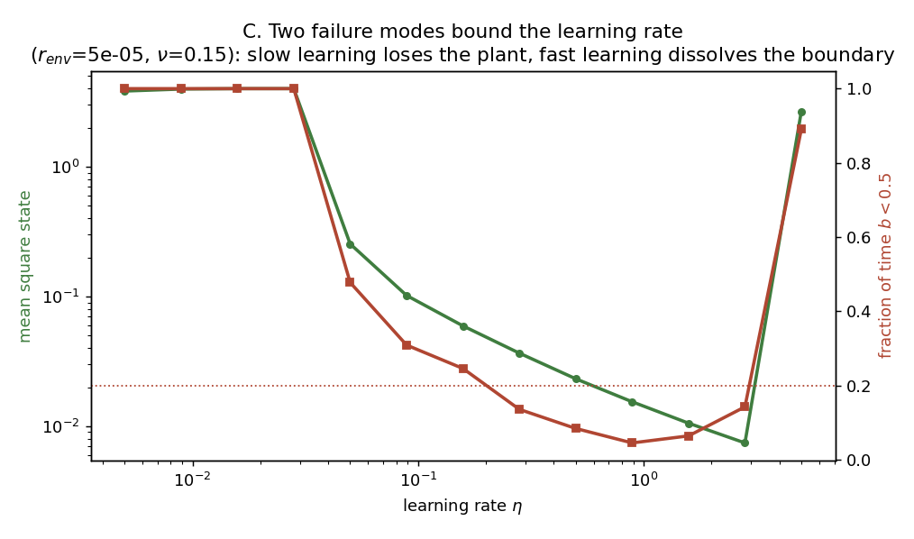
The bandwidth is not a symmetric penalty for missing an optimum. The simulation slice (Figure xviii_C_bandwidth_slice, at $r_{\text{env}}=5\times 10^{-5}$, $\nu =0.15$) shows what each violation looks like. Below ${\eta }_{\min }$, the system fails in the state: gains lag the drift, the plant saturates, non-factorizable residence is total because the wreckage is genuinely coupled. Above ${\eta }_{\max }$, the system fails in the boundary while succeeding in the state: at the fastest learning rate swept, tracking is essentially perfect — mean-square state around $0.006$ — while the system resides in the non-factorizable regime 89% of the time. Every performance dashboard is green; the separation that makes "jurisdiction" a meaningful word has dissolved. This is the boundary-domain twin of Paper XV's effective-but-self-blinding regime, produced here without any sensing saturation: the blindness is not a capacity shortfall but a structural consequence of what fast adaptation does to the decomposition it operates within. [R within the model]; the institutional reading [IP].

(Figure: xviii_C_bandwidth_slice.png — slow learning fails in the state, fast learning fails in the boundary.)

4.3 The dynamic pinch and the Decomposability Frontier (P3)

Both bounds are state-dependent, and their state-dependence points the wrong way for comfort. The numerator of ${\eta }_{\max }$ is a coupling margin, and everything that happens on the approach to collapse — the stock rising, clarity sagging, residuals growing — shrinks it. The leak term pushes ${\eta }_{\min }$ up as absorbed drift accumulates. The window therefore pinches endogenously, from both ends, fastest exactly when the system is already in trouble: the dynamic pinch. [R within the model] as comparative statics of the two formulas.

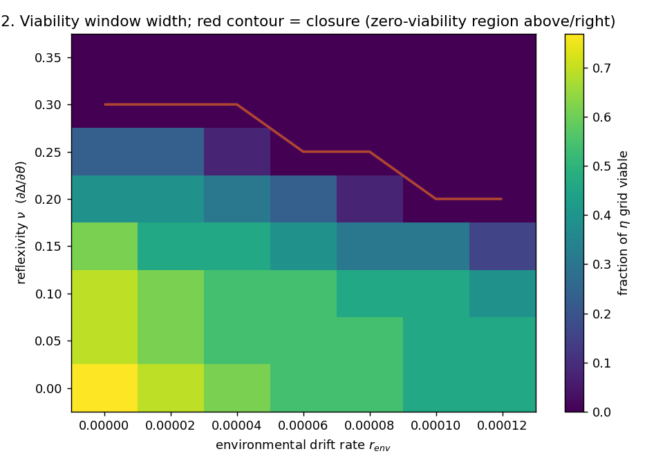
The registered prediction P3 — that the window narrows in $r_{\text{env}}$ and the reflexivity strength, and closes for some combinations — is supported. The window map (Figure xviii_C2_window_map, viability requiring bounded states, no saturation lock, and NF residence below 20% somewhere on a 13-point log-$\eta$ grid) shows the viable fraction shrinking in both coordinates and reaching zero on 36% of the $(r_{\text{env}},\nu )$ grid. The closure contour is the empirical Decomposability Frontier: past it, no learning rate exists that both tracks the environment and preserves the boundary. This is the zero-viability condition as a realized region of parameter space, not a limiting case — and it includes combinations with $r_{\text{env}}=0$, where high reflexivity alone closes the window. [R within the model.] The frontier generalizes Paper XII's Information–Actuation Frontier from a trade-off over boundary placement to a trade-off over adaptation speed, and unlike a trade-off it has an infeasible side.

(Figure: xviii_C2_window_map.png — viable window width over (r_env, ν); the red contour is the Decomposability Frontier.)

5. The Boundary Dissolution Index, revised by its own test

5.1 The registered index, and the honest test

The outline registered an early-warning claim: hidden accumulation, invisible in outcome means, would leave a fingerprint in cross-boundary prediction-error covariance, and an index ${\rho }_{\text{boundary}}$ — the largest singular value of the cross-correlation block between internal and external prediction errors, which for one monitored variable per side reduces to a rolling $|\mathrm{corr}(r_1,r_2)|$ — would rise with positive lead time before clarity collapses (P2), with the registered consequence that failure would cost §5 and §6.1 their support.

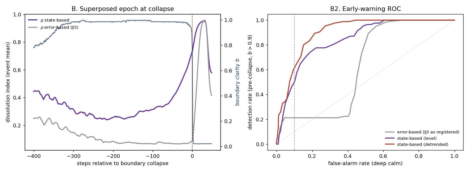
The first test appeared to deliver support, and rejecting that appearance is part of the result. A threshold-crossing count reported 86–94% of collapses "warned" with median leads near 390 steps. Its own diagnostics dismantled it: the leads approached the full cycle length, and the index sat above threshold 45% of deep-calm time — a detector that is simply often on, warning of everything and therefore of nothing. The honest instrument is a detection/false-alarm study (A.2.5): detection means exceedance in a pre-collapse window while the dashboard is still green; a false alarm is exceedance in deep calm. At a 10% false-alarm budget, over 85 events, the error-based index as registered detects 21% of collapses. Two variants defined on cross-boundary state correlation do better — 46% at the level, 60% detrended against its own trailing baseline, with median leads of 87 and 56 steps — but neither reaches a standard one would call reliable. P2 is falsified as registered, and the registered consequence binds: this section is revised, and §6.1's monitoring principle is weakened below.

(Figure: xviii_B_early_warning.png — superposed epoch at collapse and the detection/false-alarm ROC; the error-based index as registered sits near the diagonal at low false-alarm rates.)

5.2 Why the registered index had to fail: learning launders the evidence

The failure has a mechanism, and the mechanism is the most series-characteristic result in the paper. The local residual is the one signal local adaptation is actively minimizing. As coupling accumulates, each controller's gradient step absorbs the cross-boundary influence into its own gain — mis-attributing external entanglement to internal dynamics — and thereby scrubs the evidence of dissolution out of its own prediction errors, precisely during the phase an early-warning index exists to illuminate. Monitoring a well-adapted institution's forecast errors for boundary trouble is monitoring the output of a process whose job is to make those errors small. It is Goodhart's law applied to the diagnostic itself: the residual was informative about coupling only so long as nothing optimized against it, and the institution's own learning is that optimizer. [R within the model] for the comparison of detectors; [IP] for the institutional reading, which extends the series' self-blinding results — Paper XV's Simulation D showed a system blinded by saturated sensing; here the blinding requires no saturation, only competence.

The coupling remains visible where no local objective is scrubbing it: in raw cross-boundary state covariance. That is the corrected home of the index.

5.3 The revised definition, and what it can honestly promise

$${\rho }_{\text{boundary}}:={\sigma }_{\max }(\mathrm{Corr}({\mathbf{x}}_{\text{int}},{\mathbf{x}}_{\text{ext}}))\in [0,1],$$

the largest singular value of the cross-correlation block between monitored state variables inside and outside the jurisdiction — the strength of the most correlated internal–external direction, requiring no normalization and no model of either side. As ${\rho }_{\text{boundary}}\to 1$, the boundary has functionally vanished as an informational separator, whatever the formal borders say. [H] until operationalized on field data, per the series' standing rule for unmeasured indices.

Its relation to Paper XII's $B$ survives the revision in weakened form. $B$ measures realized mismatch — the variance share attributable to cross-boundary flows — and is high when the damage is already arriving; ${\rho }_{\text{boundary}}$ measures the correlational structure that precedes the damage, and in the model it rises during accumulation. They are complements: level and leading indicator. But the honest promise is now graded. Detection in the model is lead-limited — most of the discriminative signal is compressed into the fast final approach, because the compounding that drives collapse is slow until it is sudden — and even the best variant catches three collapses in five at a strict false-alarm budget. The index is a genuine improvement over outcome monitoring, which catches none of the accumulation phase at all; it is not a tripwire, and a governance architecture that treats it as one will be surprised on schedule.

Two further constraints carry over from the series. Monitoring ${\rho }_{\text{boundary}}$ spends sensing capacity, which Paper XV establishes is finite and frequently the binding stage; the prescription in §6.1 must therefore be an allocation claim, not an addition claim — some sensing must be moved from outcome tracking to boundary tracking, at a cost to the former. And the index inherits Paper X's warning about correlated observers: internal and external monitored variables measured through a shared apparatus will manufacture cross-boundary correlation that is an artifact of the sensing, not a property of the plant. The operationalization, when it comes, needs decorrelated channels on the two sides of the boundary it is trying to watch — which is, not coincidentally, the same architecture §6.4 requires for different reasons.

6. Design principles for meta-stable governance

The theorem forbids a drift-proof boundary; the model shows what drift does; the bandwidth bounds what learning may attempt. What remains designable is the margin — and the five principles below are, in the terms of §2.3, five ways of engineering the failure of the theorem's transversality hypothesis or of surviving its consequences. All five are prescriptions, not claims; the claims they rest on carry their tiers from §§2–5 and Appendix A, and each principle is scoped to world-coupled systems, where external facts resist redefinition and re-factorization is never free.

6.1 Boundary-health monitoring, as an allocation with a stated yield

Track the revised ${\rho }_{\text{boundary}}$ — cross-boundary state covariance through decorrelated channels — as a dedicated health metric distinct from outcome KPIs. The principle survives §5's falsification in weakened, and therefore honest, form. What monitoring buys is graded: in the model, the best variant detects three collapses in five at a strict false-alarm budget, with median leads short relative to the accumulation phase, because the compounding that drives collapse is slow until it is sudden. What it must never be built on is the intuitive alternative: each jurisdiction's own forecast errors, which §5.2 shows are scrubbed clean by the jurisdiction's own competence. And what it costs is sensing capacity that Paper XV establishes is finite and often binding — the prescription is to move sensing from outcome tracking to boundary tracking, accepting degraded outcome resolution as the price of any warning at all. An architecture that funds boundary monitoring only as a supplement, to be cut when outcome pressure rises, has chosen — during calm, which is when the choice is invisible — to meet the next collapse unwarned.

6.2 Oscillation damping under the friction–timescale constraint

The recovery phase of §3.2 is a panic: gains spiked against wreckage, clarity restored on suppressed symptoms, the next cycle seeded. Institutional friction — supermajorities, mandatory waiting periods, fixed review cycles — damps exactly this overcorrection, and the series' standing caution applies: friction is safe only if the timescale of hidden coupling accumulation exceeds the institutional review latency,

$${\tau }_{\text{accumulation}}>{\tau }_{\text{review}}.$$

The model now gives the left side content: ${\tau }_{\text{accumulation}}$ is set by the stock's relaxation rate $\mu$ and the distance to the fold, and it shrinks along the approach to collapse as the compounding accelerates. Friction calibrated to calm-phase accumulation speeds can therefore be safe for years and lethal in the final approach — the constraint must be evaluated against the fastest coupling the jurisdiction faces, not the average. Where coupling is driven by computational or market dynamics operating below the review latency, friction does not damp the oscillation; it guarantees that every correction arrives after the phase it was correcting has ended, which is Paper XII's spillover oscillation rebuilt inside a single jurisdiction. The constraint resolves into a design choice with no free lunch: match damping speed to coupling speed, or shrink the boundary until the couplings inside it are slow enough to damp.

6.3 Polycentricity as a decomposability reservoir

The theorem is quantified over fixed decompositions: every single $\mathbf{\Pi }$ is escaped. It says nothing against holding several. Overlapping, functionally specific jurisdictions at different scales are, in this frame, a portfolio of compatibility varieties — when the trajectory escapes one ${\mathcal{V}}_{\mathbf{\Pi }}$, it need not have escaped the others, and coordination can shift its weight toward the decompositions that currently hold. This is a reading of polycentric governance at [IP]: its value here is not subsidiarity, participation, or experimentation — the standard defenses — but structural redundancy in the space of boundaries, insurance written against a theorem. Two costs are owed to honesty. Overlap is exactly what Paper XI prices: more centers means more chains, more interfaces, more of the delegation attenuation the series has quantified — the reservoir is bought at fidelity cost, and the pooling paradox does not wave polycentric arrangements through. And the reservoir drains: each center is itself a learner, each of its boundaries drifts by the same theorem, and a polycentric order that does not renew its stock of viable decompositions is running down an inheritance. Polycentricity buys time and options; it does not buy exemption.

6.4 External certification anchors, at their own tier

Appendix A.4 proves, within the model, the two halves of the regress result. Necessity: every internal halting rule is a parameter at some level, and a hierarchy whose every level learns through coupling-relevant channels drifts at its top level — adding meta-controllers relocates the drift and never removes it; only a $\theta$-independent term of the dynamics halts it. Directional sufficiency: an anchor halts drift only in the directions it constrains, and an anchor pinning directions orthogonal to the drifting coupling satisfies the letter of "external constraint" and none of its function.

Paper XVII supplies, at [IP] and no higher, what such $\theta$-independent terms can institutionally be — and its relocation invariant is the standing warning that most apparent anchors are, on inspection, parameters at a higher level, which is precisely the regress the proposition formalizes. The design imperative is therefore XVII's own lever, adopted here without inflation: couple every jurisdiction to an epistemic signal outside its optimization manifold — independent audits, randomly sampled citizen assemblies, scientific assessment with structural firewalls, ecological telemetry — while treating each as a fallible certification link to be minimized, discretized, and cost-hardened, never as unmanipulable ground truth, which XVII establishes does not institutionally exist. A.4.2 adds the model's contribution to the placement question: the anchor must constrain the coupling-relevant directions. An audit regime that certifies budget execution while the drifting coupling runs through data-sharing interfaces is an anchor in the wrong subspace — exactly the failure §5.2 predicts for institutions that monitor what is easy rather than what is drifting.

6.5 Bandwidth governance

The Critical Learning Bandwidth is not only a finding; it is an operand. Institutions choose their learning rates — through reform frequency, pilot-program cadence, rulemaking cycles, the aggressiveness of adaptive management — and §4 says the choice has a viable window that is measurable in principle and closed in part of the parameter space. Three prescriptions follow. Locate the window before accelerating. Reform programs justified by ${\eta }_{\min }$ pressure — "the world is changing too fast for our institutions" — are half-briefed unless they also estimate ${\eta }_{\max }$: how strongly the system's own policy velocity feeds its cross-boundary coupling, the $\nu$ of §3.1, observable in principle as the coupling consequences of past rule changes. Respect the pinch. Both bounds move against the system on the approach to trouble, so a learning rate chosen in calm sits closer to the edges than its chooser believes; the margin, not the midpoint, is the design target. Treat a closed window as an architecture problem, not a calibration problem. Where the frontier of §4.3 has been crossed — where no learning rate both tracks the environment and preserves the boundary — the remedies are structural: reduce $\nu$ by insulating rule changes from boundary interfaces, reduce the coupling gain by narrowing the jurisdiction, or accept managed NF residence with the anchors of 6.4 carrying loads the boundary no longer can. Tuning $\eta$ inside a closed window is the one intervention guaranteed to fail, since the window's closure is precisely the statement that no such tuning exists.

7. Implications and structural integration

7.1 The maintained decomposability margin

The paper's reframing can now be stated with its full content behind it. The governance question inherited from Paper XII — what is the right boundary? — presupposes that rightness, once achieved, persists. The theorem removes the presupposition: every fixed boundary is escaped by generic learning, so rightness is not a state but a rate problem, and the operative question becomes how is a decomposability margin maintained under endogenous drift? The margin has now been given coordinates. It is the distance to the fold in §3's phase space; the width of the viable window in §4; the numerator of ${\eta }_{\max }$; the residual detection lead of §5; the unexhausted reservoir of §6.3. The Decomposability Frontier generalizes the Information–Actuation Frontier and adds what a static trade-off lacks: an infeasible region, reachable, and reached in the model by reflexivity alone. Every governance architecture that learns occupies a point relative to that frontier, and most are unaware the coordinate exists — which is itself a §6.1 claim about what is currently being monitored.

7.2 Unity with the series

Paper XII supplied the static boundary analysis; this paper supplies its drift dynamics. The relation is exact rather than loose: XII's Scenario (d) already showed adaptive boundaries chasing exogenous coupling change and failing beyond a critical chase rate; here the coupling change is endogenous to the chaser, which is why no chase rate suffices and the analysis must move from tracking to margin maintenance. XII's small-gain certificate is, by Corollary 1, a statement about $\theta (0)$ only.

Paper XV bounds learning from below; this paper bounds it from above; together they define the bandwidth, and the two failure modes remain distinguishable in kind — XV's is a throughput failure, this paper's a decomposition failure, and §4.2's green-dashboard regime shows a system passing every XV-style throughput test while failing the boundary completely. The leak-driven growth of ${\eta }_{\min }$ (§4.1) adds a small return contribution: holding an absorbed adaptation costs standing learning rate, so XV's lower bound rises with accumulated, not only ongoing, change.

Paper XVI established that a quantity representing unused alternatives decays under optimization and persists only through a source term the optimizer does not set. The laundering result of §5.2 is a new instance of the schema with a diagnostic twist: the decaying quantity is the informativeness of a signal — the residual's correlation with coupling — and the optimizer consuming it is the institution's own adaptation, which is why the surviving signal (cross-boundary state covariance) is precisely the one outside every local objective's control set. Source-term locality, applied to evidence.

Paper XVII and this paper exchange results at their respective tiers, in both directions. A.4.1 gives XVII's certification floor a within-model necessity proof it did not claim for itself; XVII gives A.4's exogenous anchor its institutional content and its standing warning (the relocation invariant) that apparent anchors are usually parameters one level up. Neither result inherits the other's tier, and §6.4 is written to keep it that way.

Papers V and XI locate the collapse phase in the series' compounding results: the NF excursion is the regime where architectural deficits compound multiplicatively (V) while actuation chains, now operating across a dissolved boundary, deliver interventions into dynamics they no longer model (XI) — the phase in which acting competently and acting destructively cease to be distinguishable from inside.

Paper X, finally, reaches this paper twice. The revised index of §5.3 inherits X's correlated-observer warning as an operational requirement — decorrelated channels on the two sides of the watched boundary. And the paper's own method inherits X's discipline: the falsification of P2 was produced by a registered prediction confronting a fixed external test, not by model diversity in the critique loop, which is the series' standing account of where decorrelation actually comes from.

8. Conclusion: the meta-stable governance attractor

The paper set out to remove one assumption from the series' boundary analysis — that coupling structure is exogenous to the controller — and the removal turned out to carry the section's whole weight. Once $\partial \mathbf{\Delta }/\partial \theta \ne 0$, factorizability is a compatibility variety of positive codimension, generic learning escapes it, and the boundary that was correct at design time is un-corrected by the adaptation it encloses. Permanent boundary stability is not merely difficult under learning; within the model it is structurally unavailable, and the only learning rules exempt are those confined, by construction, to boundary-respecting channels.

What replaces it is not resignation but a narrower, harder target: managed meta-stability — a regime in which the system visits factorizable phases long enough to function, and maintains the sensing, damping, redundancy, and anchoring needed to keep each visit from destroying the separability the next visit depends on. The model gives the regime its coordinates and its enemies. The reflexive cycle shows what unmanaged meta-stability looks like: calm bought on suppressed symptoms, recovery miscalibrated by the very adaptation that produced it. The locked non-factorizable regime shows the terminus past the cycle: oscillation is the intermediate case, and past a reflexivity threshold the boundary does not oscillate but welds shut. And the Critical Learning Bandwidth prices the whole arrangement: the window between learning too slowly for the world and too quickly for the boundary is real, state-dependent, pinched from both ends on the approach to trouble, and closed outright on a substantial region of parameter space — the Decomposability Frontier, a constraint with an infeasible side, which no calibration crosses and only architecture can move.

The paper's most instructive result was not registered but forced. The Boundary Dissolution Index, defined as the outline defined it, failed its own test, and the failure had a mechanism worth more than the index: local adaptation absorbs cross-boundary influence into internal gain and thereby launders the evidence of dissolution out of exactly the residuals a well-run institution watches. The signal that survives is the one no local objective controls. A series about the limits of institutional perception should perhaps have predicted that its own proposed instrument would be subject to them; that it did not, and that the registered-prediction discipline caught it, is the method working as designed.

The reframing, then, in one sentence: the governance question is not where to draw the boundary, but how to maintain a decomposability margin under the drift that learning inevitably induces — and the five principles of §6 are the current, avowedly partial, answer to what maintaining one requires.

9. What this paper does not show

The discipline of the cluster applies to its own results, and the refusals are load-bearing.

It does not show that boundary drift is universal. The theorem is scoped twice. Formally, it is conditional on transversality: learning confined to boundary-respecting channels preserves factorizability indefinitely, and §6 is an attempt to engineer exactly that. Substantively, the reflexivity asymmetry of §1.4 exempts self-referential coordination, where re-factorization is free because the facts on both sides of a boundary are conventions; the exemption is an argument, not a corollary, and it inherits Paper XVII's scope bound at [IP].

It does not show that the four-phase cycle is the unique dynamics. The simulation itself exhibits three regimes, and the cycle is the intermediate one; other model specifications may produce others. The claim established is existence in a non-degenerate parameter region, not typicality across institutions, and the phase narrative is a description of the model's cycling regime carrying an [IP] institutional gloss, not a stage theory of institutional history.

It offers no field instrument. Every quantity the paper turns on — $\partial \mathbf{\Delta }/\partial \theta$, the coupling stock, ${\epsilon }_{\text{crit}}$, the window bounds, ${\rho }_{\text{boundary}}$ itself — is defined within the model and measured nowhere. The revised index is [H] until operationalized, and §5.3's constraints (sensing allocation, decorrelated channels) are conditions on an operationalization that does not yet exist. The bandwidth formulas are averaged results whose institutional analogues would require estimating quantities current monitoring architectures are not built to collect — the same admission Paper XII made for $B$, owed again here.

It does not establish the early-warning value of boundary monitoring; it bounds it. P2 failed as registered. The state-based variants detect three collapses in five at a strict false-alarm budget, with short leads; the honest claim of §6.1 is that monitoring the right signal is graded insurance, not a tripwire, and any stronger claim died in this paper's own event study.

It does not strengthen Paper XVII. A.4.1 proves necessity of an exogenous anchor within a linear model; the certification floor remains [IP], its evidence remains concept-isomorphism, and the relocation invariant remains a warning rather than a theorem. Nothing here converts institutional certification into ground truth — the opposite: A.4.2 shows that even a genuine anchor is useless in the wrong subspace.

It does not license the frontier as a diagnosis of any actual polity. The Decomposability Frontier is a realized region of the model's parameter space. Whether any existing governance system sits near or past its institutional analogue is an empirical question the paper is not equipped to answer, and locating one there by narrative resemblance — the temptation the result most invites — is precisely the promotion of a regime-conditioned pattern into a law that the cluster's standing rule forbids.

And it does not close the design question it opens. The five principles maintain a margin; none of them manufactures one where the window has closed. What institutional forms can operate durably past the frontier — under managed non-factorizability, with anchors carrying loads that boundaries no longer can — is the question this paper ends on and does not answer.

(Simulation: paper_xviii_boundary_instability.py, seed 20260703; all quoted numbers are printed by its verification block. Registered predictions and their outcomes: P1 supported, P2 falsified as registered, P3 supported.)

Appendix A — Formal Development and Simulation

Conventions. Tiers follow the series: [R] rigorous, [IP] in principle, [H] heuristic; "[R within the model]" marks results that are exact or proven for the stated formal model, with no claim beyond it. All matrix-derivative statements use the Frobenius inner product on vectorised operators, ${⟨U,V⟩}_F=\mathrm{tr}(U^{\top }V)$ on $\mathrm{vec}(\cdot )$. The simulation is paper_xviii_boundary_instability.py, seed 20260703; every number quoted in this appendix is printed by that script's verification block. Figures referenced: xviii_A_phase_cycle, xviii_A2_regime_map, xviii_B_early_warning, xviii_C_bandwidth_slice, xviii_C2_window_map.

A.1 The Non-Factorizability Theorem via common invariant subspaces

A.1.1 Setup

State $\mathbf{x}\in {\mathbb{R}}^n$, parameters $\theta \in \Theta \subseteq {\mathbb{R}}^p$, dynamics $\mathbf{x}(t+1)=\mathbf{A}(\theta (t))\mathbf{x}(t)$ with $\mathbf{A}$ smooth in $\theta$, and learning $\theta (t+1)=\theta (t)+\eta \mathbf{L}(\mathbf{x}(t),\theta (t))$, $\eta >0$. A jurisdictional split is an orthogonal decomposition ${\mathbb{R}}^n=\mathcal{S}\oplus {\mathcal{S}}^{\perp }$ with $\dim \mathcal{S}=d$, $0<d<n$, and projection $\mathbf{\Pi }$ onto $\mathcal{S}$.

Definition (factorizability). The split $\mathbf{\Pi }$ factorizes the dynamics at $\theta$ if both blocks of cross-influence vanish: $$\mathbf{\Pi }\mathbf{A}(\theta )(\mathbf{I}-\mathbf{\Pi })=0\text{and}(\mathbf{I}-\mathbf{\Pi })\mathbf{A}(\theta )\mathbf{\Pi }=0,$$ i.e. both $\mathcal{S}$ and ${\mathcal{S}}^{\perp }$ are invariant subspaces of $\mathbf{A}(\theta )$. (The weaker block-triangular condition — one invariant subspace, one-way influence — admits an exactly analogous treatment; governance separation in the sense of Paper XII requires the two-sided form, and we state everything for it.) A fixed decomposition along a trajectory is a single $\mathbf{\Pi }$ factorizing $\mathbf{A}(\theta (t))$ for all $t$: a common invariant-subspace pair of the matrix family $\{\mathbf{A}(\theta (t)){\}}_t$.

For fixed $\mathbf{\Pi }$ define the compatibility variety $${\mathcal{V}}_{\mathbf{\Pi }}=\{\theta \in \Theta :\mathbf{\Pi A}(\theta )(\mathbf{I}-\mathbf{\Pi })=0,(\mathbf{I}-\mathbf{\Pi })\mathbf{A}(\theta )\mathbf{\Pi }=0\},$$ the zero set of $2d(n-d)$ smooth scalar functions of $\theta$. Factorizability along the trajectory is exactly confinement: $\theta (t)\in {\mathcal{V}}_{\mathbf{\Pi }}$ for all $t$.

Definition (coupling sensitivity). $\partial \mathbf{\Delta }/\partial \theta$ denotes the derivative of the off-diagonal blocks, i.e. of the map $\theta \mapsto (\mathbf{\Pi A}(\theta )(\mathbf{I}-\mathbf{\Pi }),(\mathbf{I}-\mathbf{\Pi })\mathbf{A}(\theta )\mathbf{\Pi })$, as a linear map ${\mathbb{R}}^p\to {\mathbb{R}}^{2d(n-d)}$ under vectorisation.

A.1.2 Theorem

Theorem A.1 (Non-Factorizability, [R within the model]). Fix a split $\mathbf{\Pi }$ and suppose:

(i) Non-degeneracy. $\partial \mathbf{\Delta }/\partial \theta$ has rank $\ge 1$ at every point of ${\mathcal{V}}_{\mathbf{\Pi }}$ visited by the trajectory, so that ${\mathcal{V}}_{\mathbf{\Pi }}$ is locally a submanifold of $\Theta$ of codimension $\ge 1$.

(ii) Transversality. The averaged learning field $\bar{\mathbf{L}}(\theta )={\mathbb{E}}_{\mathbf{x}}[\mathbf{L}(\mathbf{x},\theta )]$ is not tangent to ${\mathcal{V}}_{\mathbf{\Pi }}$ on any relatively open subset of ${\mathcal{V}}_{\mathbf{\Pi }}$: equivalently, ${⟨\partial \mathbf{\Delta }/\partial \theta [\bar{\mathbf{L}}(\theta )],\cdot ⟩}_F\not\equiv 0$ there.

(iii) Persistence. The trajectory does not converge to a stationary point of the learning dynamics lying inside ${\mathcal{V}}_{\mathbf{\Pi }}$.

Then $\theta (t)$ leaves ${\mathcal{V}}_{\mathbf{\Pi }}$ in finite time. Since the argument holds for every admissible split, no fixed decomposition of the state space remains exact along a learning trajectory satisfying (i)–(iii): factorizability is not a structural invariant of the learning system but a trajectory-dependent, transient property.

Stochastic form. If the learning update carries noise whose distribution is absolutely continuous on ${\mathbb{R}}^p$ (as in the simulation, where $\mathbf{L}$ inherits the process noise through $\mathbf{x}$), then escape from ${\mathcal{V}}_{\mathbf{\Pi }}$ is almost sure regardless of (ii), since ${\mathcal{V}}_{\mathbf{\Pi }}$ has Lebesgue measure zero under (i) and the one-step transition kernel assigns it probability zero. The deterministic statement uses transversality; the stochastic statement uses measure. The paper uses whichever hypothesis matches the setting and does not mix the vocabularies.

Proof. Suppose $\theta (t)\in {\mathcal{V}}_{\mathbf{\Pi }}$ for all $t$. Then every increment $\theta (t+1)-\theta (t)=\eta \mathbf{L}$ connects points of ${\mathcal{V}}_{\mathbf{\Pi }}$; passing to the averaged flow (valid for $\eta$ small on the relevant horizon; for the discrete argument replace tangency by "increments stay in a tubular neighbourhood shrinking with $\eta$"), confinement requires $\bar{\mathbf{L}}(\theta (t))\in T_{\theta (t)}{\mathcal{V}}_{\mathbf{\Pi }}$ along the whole visited set. By (iii) the visited set is not a single stationary point, hence contains a relatively open piece of an orbit in ${\mathcal{V}}_{\mathbf{\Pi }}$; (ii) denies tangency on any such piece. Contradiction; the trajectory exits. The stochastic case is immediate from absolute continuity. $\square$

A.1.3 What the theorem does and does not say

Three deliberate restraints. First, the theorem is conditional on (ii): a learning rule constructed to act only through block-respecting channels — $\bar{\mathbf{L}}\in T{\mathcal{V}}_{\mathbf{\Pi }}$ by design — preserves factorizability forever. The content of the theorem is that this alignment is a codimension condition, not a default: generic learning that acts through any coupling-relevant channel breaks every fixed split. The design principles of §6 are, in this exact sense, attempts to engineer (ii)'s failure — to constrain learning into the tangent bundle of a chosen decomposition. Second, "leaves ${\mathcal{V}}_{\mathbf{\Pi }}$" means the decomposition ceases to be exact; how fast the off-diagonal blocks then grow, and whether the M–Δ loop gain of Paper XII crosses unity, is a quantitative question the theorem does not answer — that is the work of §A.2–A.3. Third, the scope asymmetry of §1 enters here and not as a corollary: nothing in the mathematics prevents (i)–(iii) from holding in a self-referential symbolic system. The asymmetry is that such a system may redefine $\mathbf{\Pi }$ by convention as the trajectory moves — re-factorization is free when the facts on both sides of the split are conventions — whereas a world-coupled system must compensate drift it cannot rename. Escape from a fixed ${\mathcal{V}}_{\mathbf{\Pi }}$ is a theorem; the cost of re-fixing $\mathbf{\Pi }$ is what separates the domains. [IP] for the domain separation, per Paper XVII's scope bound.

Corollary A.1.1 (Spectral drift, [R within the model]). Any stability certificate evaluated at $\theta (0)$ — in particular the small-gain condition $\Vert \mathbf{M}\Vert \Vert \mathbf{\Delta }\Vert <1$ of Paper XII — is not invariant under learning satisfying (i)–(iii). Stability is a property of the joint (plant + controller + learning rule) trajectory.

Corollary A.1.2 (Environment as field, [R within the model]). Along such a trajectory $\mathbf{\Delta }=\mathbf{\Delta }(\theta (t))$ is a policy-dependent interaction field; treating it as an exogenous operator mis-specifies the stability problem from the first step.

A.2 The reflexive boundary cycle: reduction and simulation

A.2.1 The model

As specified in §3.1, with the implementation choices declared there and in the simulator header: two scalar subsystems $$x_i(t+1)=(a_t-k_i)x_i+\epsilon (t)x_j+w_i,w_i\sim \mathcal{N}(0,{\sigma }_w^2),$$ soft-saturated at $X_{\text{sat}}$; coupling $\epsilon ={\epsilon }_0+\alpha (1-b)+\beta c$ with the stock $c(t+1)=(1-\mu )c+\mu x_1{x}_2+\nu (|\Delta k_1|+|\Delta k_2|)$; closed-model residuals $r_i=x_i(t+1)-(a_0-k_i)x_i=(a_t-a_0)x_i+\epsilon x_j+w_i$; gradient learning with leak, $k_i\leftarrow (1-\lambda )k_i+\eta x_i{r}_i$; boundary clarity $b\leftarrow \sigma (\gamma (1-\overline{|r|}/R)-\delta |\epsilon |+h(b-\frac{1}{2}))$. Note two structural facts that the reduction uses. The residual is independent of $k_i$: each local model carries its own gain correctly, so what learning sees is exactly the unmodeled content — drift staleness plus coupling plus noise. And $\theta =(k_1,k_2)$ reaches $\mathbf{\Delta }$ through two channels: indirectly through the states (the $\mu x_1{x}_2$ term) and directly through policy velocity (the $\nu$ term), the latter being the model's literal $\partial \mathbf{\Delta }/\partial \theta \ne 0$.

A.2.2 Fast-subsystem statistics in closed form

Hold $(\epsilon ,k_1=k_2=k,b)$ fixed and take the unsaturated linear regime. In the mode coordinates $s=(x_1+x_2)/\sqrt{2}$, $d=(x_1-x_2)/\sqrt{2}$ the dynamics decouple with poles $p_{\pm }=a-k\pm \epsilon$, giving stationary variances ${\sigma }_w^2/(1-p_{\pm }^2)$ and hence, exactly, $$q(\epsilon ,k):=\mathbb{E}[x_1{x}_2]=\frac{{\sigma }_w^2}{2}\left[\frac{1}{1-p_{+}^2}-\frac{1}{1-p_{-}^2}\right],{\sigma }_x^2=\frac{{\sigma }_w^2}{2}\left[\frac{1}{1-p_{+}^2}+\frac{1}{1-p_{-}^2}\right].$$ [R within the model.] $q$ is positive for $\epsilon >0$, increasing in $\epsilon$, and diverges as $p_{+}\to 1$: the symmetric mode loses stability at $${\epsilon }_{\text{inst}}(k)=1-(a-k),$$ the line marked in Figure xviii_A_phase_cycle. This divergence is the collapse mechanism: the interaction statistic that feeds the stock blows up precisely as the coupling approaches the margin the local gains leave open.

A.2.3 The averaged slow system and the anatomy of the cycle

The timescale separation in the calm phase is roughly: fast states (mixing time $(1-|p_{\pm }|{)}^{-1}\sim 10$–$25$ steps), slow stock (${\mu }^{-1}=50$), slow gains (${\lambda }^{-1}=100$), with $b$ a fast switch slaved to $(\overline{|r|},\epsilon )$ except in its bistable band. Averaging over the fast states (replace $x$-statistics by their stationary values) yields a planar slow system in $(c,b)$ with the gains slaved by the learning–leak balance $\lambda k^{\ast }=\eta [(a_t-a_0){\sigma }_x^2+\epsilon q]$: $$c^{+}=(1-\mu )c+\mu q(\epsilon (c,b),k^{\ast })+2\nu \eta \mathbb{E}|x_i{r}_i|,b^{+}=\sigma \left(\gamma \right(1-\frac{\mathbb{E}|r|}{R})-\delta \epsilon (c,b)+h(b-\frac{1}{2})),$$ with $\mathbb{E}|r|\approx \sqrt{2/\pi }({\epsilon }^2{\sigma }_x^2+{\sigma }_w^2{)}^{1/2}$ and $\mathbb{E}|x_i{r}_i|\approx (2/\pi ){\sigma }_x{\sigma }_r$ up to a correlation-dependent factor of order one (the simulation, not these approximations, carries the quantitative burden).

The relaxation-oscillation anatomy is read directly off this pair. On the clear branch ($b\approx 1$) the stock ramps slowly toward the $q$-divergence — hidden accumulation, hidden because $\mathbb{E}|r|$ grows only with ${\epsilon }^2$ while $q$'s feedback is compounding. The divergence of $q$ is the fold: $c$ and $\epsilon$ run away on the fast timescale — collapse — until saturation bounds the excursion and the now-large learning signal drives $k$ up on what has become a fast timescale, violating the separation; the averaged system is therefore valid in the accumulation phase and heuristic across the excursion, and we say so rather than claim otherwise. High $\overline{|r|}$ and $|\epsilon |$ throw $b$ to its dissolved branch. Gain growth kills $q$; the stock decays; calm returns; $b$'s memory term releases; the leak then bleeds $k$ back down, re-arming the instability — miscalibrated re-entry. A rigorous limit-cycle proof would require the continuous-time planar limit of the averaged map, a verified trapping region, and Poincaré–Bendixson on that reduction; we do not claim it. The reduction explains the cycle's anatomy [R within the model] for A.2.2's statistics and [H] for the excursion phase; existence of the cycle is established numerically.

A.2.4 Simulation results: P1

Exhibit run ($T=6000$, baseline parameters): 9 collapse–recovery events, with the four phases visible in Figure xviii_A_phase_cycle — the stock ramp below a quiet $b$, the $\epsilon$ excursion past $1-a_0$, the gain spike, the $b$ collapse and staggered recovery. Regime map (Figure xviii_A2_regime_map; $12\times 12$ grid, $\beta \in [0.2,2.4]$, $\eta \in [0.005,0.5]$ log-spaced, 2 seeds): 36% of the grid sustains the cycle. The cycling region is bounded on one side by a quiescent regime (reflexivity too weak to reach the fold) and on the other by a locked non-factorizable regime, not anticipated in the outline and reported as a finding: at high $\beta$, the post-collapse coupling floor ${\epsilon }_0+\alpha (1-b)$ is itself high enough to hold $b$ at zero permanently — the boundary never recovers, and the system settles into permanent NF residence rather than oscillation. P1: supported — a sustained oscillation exists in a non-degenerate parameter region, and the four-phase narrative of §3.2 describes it; the narrative must additionally acknowledge the locked regime as the cycle's high-reflexivity terminus. [R within the model.]

A.2.5 Simulation results: P2, and the failure of the registered index

The registered index — ${\rho }_{\text{boundary}}$ as the largest singular value of the cross-boundary prediction-error correlation block, here with one monitored variable per side reducing to $|\text{rolling corr}(r_1,r_2)|$, window 150 — was tested against a state-based variant $|\text{rolling corr}(x_1,x_2)|$ and its detrended form (level minus trailing 400-step median). A first, naive test (threshold-crossing counts) appeared to support both variants — 86–94% of events "warned", median leads $\approx$ 390 steps — and was rejected by its own diagnostics: the leads approached the full cycle length, and the state-based index sat above threshold 45% of deep-calm time. An index that is simply "often on" warns of everything and therefore of nothing. The honest instrument is a detection/false-alarm study: detection = exceedance in $[t_0-300,t_0-10]$ before a collapse at $t_0$ while the dashboard is still green ($b>0.9$); false alarm = exceedance in deep calm ($b>0.9$, $>400$ steps from the next collapse). Over 85 events, at a false-alarm budget of 10% (Figure xviii_B_early_warning):

P2: falsified as registered. The registered consequence binds: §5 is revised, and §6.1's monitoring principle is weakened to a graded claim. The mechanism of the failure is itself a result, and arguably the most series-characteristic one in the paper: the local residual is the one signal local adaptation is actively minimising. Learning absorbs the coupling into gain, so the evidence of boundary dissolution is laundered out of each side's own prediction errors precisely during the phase an early-warning index is supposed to illuminate — Goodhart's law applied to the diagnostic itself, and the dynamic kin of Paper XV's effective-but-self-blinding regime. The coupling remains visible where no local objective is scrubbing it: in the raw cross-boundary state covariance. Even there the discrimination is partial (0.46–0.60 at strict budgets), because the accumulation's final approach is fast — most of the discriminative signal is compressed into the last $\sim$100 steps. The revised §5 must therefore (a) define ${\rho }_{\text{boundary}}$ on cross-boundary state covariances, (b) state the laundering result as the reason error-based monitoring is structurally misleading, and (c) present boundary-health monitoring as lead-limited rather than as a reliable tripwire. [R within the model] for the comparison; [IP] for the institutional reading.

A.3 The Critical Learning Bandwidth

A.3.1 The lower bound

Under drift $a_t=a_0+r_{\text{env}}t$, the residual is $r_i=(a_t-a_0)x_i+\epsilon x_j+w_i$, so the averaged gain flow is $$\dot{k}=-\lambda k+\eta [(a_t-a_0){\sigma }_x^2+\epsilon q].$$ Write $e_k=(a_t-a_0)-k$ for the un-absorbed drift; the effective pole is $a_0+e_k$ (plus coupling), and viability requires $e_k<m:=1-a_0-\epsilon -$ (stability margin). On the ramp-following solution $\dot{k}\approx r_{\text{env}}$, $$e_k\approx \frac{r_{\text{env}}+\lambda (a_t-a_0)}{\eta {\sigma }_x^2},\text{hence}{\eta }_{\min }(t)\approx \frac{r_{\text{env}}+\lambda (a_t-a_0)}{{\sigma }_x^{2}m}.$$ [R within the model] for the averaged balance. Two readings. The drift rate enters as expected — this is Paper XV's lower bound in local form. Less expected: the leak term makes ${\eta }_{\min }$ grow with the accumulated drift $(a_t-a_0)$ even at constant $r_{\text{env}}$ — with decaying authority, merely holding an absorbed adaptation costs learning rate. When slow learning fails, it fails through state divergence: in the sweep at $(r_{\text{env}},\nu )=(5\times 10^{-5},0.15)$, the slow end shows saturation lock and NF residence 1.00.

A.3.2 The upper bound

Fast learning fails through the direct reflexive channel. In calm, the expected policy velocity is $\mathbb{E}|\Delta k_i|=\eta \mathbb{E}|x_i{r}_i|\approx (2/\pi )\eta {\sigma }_x{\sigma }_r$, so the stock equilibrates at $$c^{\ast }=q+\frac{2\nu \eta }{\mu }\mathbb{E}|x_i{r}_i|,$$ and the clear branch of the boundary switch survives only while $\epsilon (c^{\ast })={\epsilon }_0+\beta c^{\ast }<{\epsilon }_{\text{crit}}$, where ${\epsilon }_{\text{crit}}(\overline{|r|}):={\delta }^{-1}[\gamma (1-\overline{|r|}/R)+h/2-s^{-1}\ln \frac{b_h}{1-b_h}]$ is the coupling at which the high fixed point $b_h$ of the sigmoid disappears. Solving, $$\boxed{{\eta }_{\max }\approx \frac{\mu ({\epsilon }_{\text{crit}}-{\epsilon }_0-\beta q)}{2\nu \beta \mathbb{E}|x_i{r}_i|/\eta }=\frac{\mu ({\epsilon }_{\text{crit}}-{\epsilon }_0-\beta q)}{(4/\pi )\nu \beta {\sigma }_x{\sigma }_r}}$$ [R within the model], averaged. The structure is the transposed slow-adaptation condition of adaptive control: adaptation must be slow relative to the timescale on which its own activity re-shapes the unmodeled dynamics — here, slow relative to the stock's relaxation $\mu$ scaled by the reflexive gain $\nu \beta$. The Rohrs precedent (§4) is cited for the structural insight, not the formula; the formula is this model's own. The empirical signature at the fast end is the distinctive one: at $\eta =5$ the system tracks perfectly (mean-square state $\sim 0.006$) while residing in NF 89% of the time — a green dashboard over a dissolved boundary, the boundary-domain twin of Paper XV's Simulation D.

A.3.3 The dynamic pinch and the closure of the window

The numerator of ${\eta }_{\max }$ is a coupling margin, and it is state-dependent: accumulation raises $q$, boundary sag raises $\epsilon$ through $\alpha (1-b)$ and raises $\overline{|r|}$, all of which shrink $({\epsilon }_{\text{crit}}-{\epsilon }_0-\beta q)$. So ${\eta }_{\max }$ falls as the system drifts toward the fold — while ${\eta }_{\min }$ rises with accumulated drift through the leak term. The window pinches endogenously, from both ends, fastest exactly when the system is already in trouble. [R within the model] for the comparative statics of the two formulas.

Simulation results: P3. Slice at $(r_{\text{env}},\nu )=(5\times 10^{-5},0.15)$, Figure xviii_C_bandwidth_slice: NF residence is 1.00 at the slow end, falls to a minimum of 0.05 in the interior, rises to 0.89 at the fast end — the two failure modes are distinct in kind (state failure vs boundary failure), not just in direction. Window map over $(r_{\text{env}},\nu )$, Figure xviii_C2_window_map (viability = saturation fraction $<0.05$, mean-square state $<0.5$, NF residence $<0.2$, over a 13-point log-$\eta$ grid): the viable window narrows in both coordinates and closes on 36% of the grid; the closure contour is the empirical Decomposability Frontier. P3: supported. Zero-viability is a realised region of parameter space, not a limiting case. [R within the model.]

A.4 Regress termination within the model

Consider a hierarchy: level 0 holds the base parameters ${\theta }^{(0)}=(k_1,k_2)$; level 1 holds meta-parameters ${\theta }^{(1)}$ (e.g. the learning rate, the leak, the boundary thresholds) adjusted by a meta-learning rule on level-0 performance; and so on to level $M$. Every internal "halting rule" — a cap, a constitution, a review threshold — is, by construction, a component of some ${\theta }^{(m)}$.

Proposition A.4.1 (Necessity, [R within the model]). If at level $m$ the meta-learning rule satisfies hypotheses (i)–(iii) of Theorem A.1 with respect to the coupling-relevant directions of ${\theta }^{(m)}$ — its adjustments have a nonzero projection, direct or through the states, onto $\partial \mathbf{\Delta }/\partial {\theta }^{(m)}$ — then boundary drift recurs at level $m$. By induction, a hierarchy whose every level learns through coupling-relevant channels exhibits drift at its top level; adding levels relocates the drift, it does not remove it. Only a $\theta$-independent term of the dynamics — a constraint not adjustable at any level — halts drift.

Proposition A.4.2 (Directional sufficiency, [R within the model]). A $\theta$-independent anchor is a submanifold ${\Theta }_{\text{anch}}\subset \Theta$ onto whose tangent bundle the learning field is projected. The anchor prevents escape from ${\mathcal{V}}_{\mathbf{\Pi }}$ iff the normal directions of ${\mathcal{V}}_{\mathbf{\Pi }}$ excited by the learning field are among the directions the anchor constrains. Sufficiency is directional: drift continues freely in the unconstrained complement. An anchor that pins the wrong directions changes nothing.

The relation to Paper XVII is one of tier-disciplined citation in both directions. Proposition A.4.1 is this model's own result: within the formalism, an exogenous term is necessary to halt meta-adaptive drift. Paper XVII's certification floor is the [IP]-tier, cross-disciplinary identification of what such exogenous terms can institutionally be — and its relocation invariant is the standing warning that most apparent anchors are, on inspection, parameters at a higher level, which is precisely the regress A.4.1 formalizes. Its design lever — minimize, discretize, and cost-harden the certification link — is what §6.4 adopts. Neither result inherits the other's tier: the proposition does not make the certification floor [R], and the floor's institutional breadth does not extend the proposition beyond the linear model. A.4.2's directionality condition is the model-level content behind §6.4's requirement that anchors constrain the coupling-relevant directions: an audit that certifies a variable orthogonal to the drifting coupling satisfies the letter of "external anchor" and none of its function.