Abstract

The Governance as Engineering series established, across its second cycle, that a viable governance architecture must do three things to remain adequate to a changing environment: sense reality through observers decorrelated enough to catch the error they share (Paper X), learn from what it senses by exploring enough to keep its model identifiable (Paper XIV), and execute its adaptation while it still retains the transition bandwidth to carry the change (Paper IX). These three requirements were established separately and ordered into a dependency — the adaptation triad, Sense → Learn → Execute — but they were never posed as three simultaneous claims on the same finite capacity. This paper closes that gap and adds no primitive. It treats the triad as what it structurally is: a recursive feedback loop, inherited from the series' founding premise that governance observes, decides, acts, and observes again (Paper I), in which execution changes the world that sensing must re-observe. The loop has finite throughput at each stage, and its two interior legs — sensing to learning, learning to execution — are lossy conversions whose efficiencies fall below one for reasons the series has already established: the aggregation loss of Paper III, and the immune-system, transition-bandwidth, and delegation attenuations of Papers VII, IX, and XI. The central result is the adaptation bottleneck theorem: the effective adaptive rate of the loop is gated by its slowest stage, so capacity added to any non-bottleneck stage does not accelerate adaptation — it accumulates as backlog. [R within the model.] Three backlogs follow, one on each leg of the loop: an information backlog when sensing outruns learning (analysis paralysis), an innovation backlog when learning outruns execution (permanent experimentation), and a reality backlog when execution outruns re-observation (rigid, confident action on a model the system's own activity has rendered stale). The third is definable only because the loop closes, and it is a rate mismatch rather than a conversion loss — the distinguishing yield of treating the triad as recursive rather than serial. The paper states the theorem, grounds the two conversion losses in the series' prior results, gives each backlog its inherited governance evidence, demonstrates the bottleneck logic in simulation, and defers two deeper questions to later work: the interference version, in which the three legs disturb rather than merely queue behind one another, and the ecology of multiple co-adapting architectures. It is the dynamic dual of Paper V — where V showed that static architectural deficits compound multiplicatively, this paper shows that dynamic adaptive capacities are gated by their minimum — and with that pairing the second cycle's internal logic is complete. What the paper does not supply is the rate at any real stage, the correct balance in any real case, or an instrument to measure either; those it leaves, in the series' standing manner, to the empirical phase.

Part I — The Problem: The Triad Was Never Costed

1.1 A Model That Outran Its Own Re-Observation

Author's note: this vignette is built on the 2007–08 financial crisis as a reality-backlog instance and is kept deliberately qualitative — no figures, no specific institutional claims requiring a source. Verify the case against your own reading, or substitute one you can stand behind, before publication.

Before the financial crisis of 2007–08, the institutions at its centre were not under-observed. They were, by the standards of any prior era, saturated with instrumentation. Risk was modelled continuously; positions were marked, stress-tested, and reported on cycles measured in days and sometimes minutes; ratings agencies, internal risk desks, and regulators all maintained apparatus whose explicit purpose was to keep the picture current. Nor were these institutions slow to act. They could move capital, rebalance exposure, and write new instruments at a speed that earlier finance could not have imagined. By the measures this series cares about, the sensing leg was richly resourced and the execution leg was fast.

What failed sat between, and behind. The models that converted observation into a working picture of risk had stopped tracking the reality that the institutions' own execution was creating: as leverage and exposure to the same correlated assets rose, the correlations themselves shifted, in a way the models — calibrated on a quieter world — could not see and were not built to re-learn quickly. The system was executing on a model it was not re-observing fast enough to keep honest, and because each fast action changed the world that the next observation would have had to capture, the gap between the world-as-modelled and the world-as-made widened silently. There was no shortage of data and no shortage of speed. There was a backlog: of reality, unobserved, accumulating behind a model that everyone trusted precisely because the dashboards in front of it were green. When the catch-up finally came, it came all at once, under the worst conditions, in the manner this series has documented at other scales — Paper XIV's crisis-driven learning, Paper VII's boom-and-bust cases, and, at the scale of a single life, the midlife reckoning of Self II.

The lesson is not that the institutions sensed too little or acted too much in any budgetary sense. More risk modelling would not have helped; faster execution would have made it worse. The lesson is about rates. A system can carry abundant capacity at two of the three stages of its adaptive loop and still fail, because adaptation is not the sum of what the stages do separately — it is what survives passage through all three in sequence, and around the loop again. That is the phenomenon this paper formalises.

1.2 The Series in One Page

The series treats a governance system as a controller in a loop with the world it governs: it observes the world's state through a channel that selects some dimensions and drops others, decides on the basis of what it observes, acts, and observes the result. Its first cycle established the static architecture of that loop — the structural primitives a system has whether or not it is changing. Latency and signal fidelity place hard ceilings on responsiveness (I); a single-speed architecture is mismatched to disturbances that arrive at many frequencies (II); representation chains attenuate the citizen-preference signal until, beyond a critical depth, the policy layer cannot reconstruct it (III, constitutional unobservability); requisite variety must live at the point of contact (IV); these deficits compound multiplicatively rather than additively (V); objective functions are themselves observation architectures, so that what a system does not value it ceases to see (VI, the variety gap); reform is absorbed by the architectures it targets unless it can open a protected experimental space (VII); and the variety gap can be made estimable (VIII). Paper XI later closed the static grammar by treating the actuation channel as the dual of III's observation channel: a directive descending a delegation chain is attenuated by each layer, yielding constitutional uncontrollability and an energy law of reform exhaustion.

The second cycle established the dynamics of adaptation — how an architecture changes, learns, and stays viable. Its results converge on a single sequence, the adaptation triad:

Sense  →  Learn  →  Execute

Sense (Paper X) is keeping observers decorrelated enough to catch the error they share — agreement among identical observers is not evidence. Learn (Paper XIV) is exploring enough to keep the system's model of the world identifiable — the rigorous content of persistent excitation. Execute (Paper IX) is retaining enough transition bandwidth to change the architecture before the window closes. The triad's logic is a dependency: a system that cannot sense reality cannot learn from it; one that cannot learn cannot adapt; one that cannot execute its adaptation cannot survive.

What the triad has not been given is a cost. Each leg was established as a requirement, and the legs were ordered into a dependency, but they have never been treated as three simultaneous claims on one finite capacity. The dependency tells us the legs must occur in order; it does not tell us what happens when they must occur together, drawing on processing capacity that no single stage can monopolise without starving the others. That is the question this paper takes up, and it is the last question the second cycle's internal logic raises about itself.

1.3 What the Triad Papers Did, and What They Left

Papers X, XIV, and IX each established their leg's requirement in isolation, and each did so well. Paper X derived the ensemble-variance result — that distributed sensing fails through correlation rather than individual error — and established that a few genuinely independent observers buy most of the available protection. Paper IX modelled architectural change as contested control and identified transition bandwidth as a race that can be lost before it is visible. Paper XIV came closest to the question this paper asks: its dual-control framework formalises the tension between exploitation (acting optimally on the current model) and exploration (acting to improve the model), shows that a single controller cannot maximise both at once, and prescribes ring-fenced curiosity budgets and the functional separation of the two.

But Paper XIV's tension is two-way and lives inside the Learn leg. It is the trade-off between using the model and improving it — a trade-off the controller faces in choosing each action. It is not the three-way question of how a system that must sense, learn, and execute, all at finite and unequal rates, allocates a loop's worth of throughput across all three stages at once. The triad papers, read together, leave a precise gap: they tell us each leg must be adequate, and they tell us the legs depend on one another in sequence, but they do not tell us that the three legs are coupled by throughput — that capacity poured into one cannot substitute for a shortfall in another, and that the loop's adaptive rate is therefore set not by the sum of the three but by the least of them. Closing that gap requires no new primitive. It requires only that the triad already established be treated as a loop with finite throughput, and the consequences read off.

1.4 The Dual of Paper V, and Three Traditions

The result this paper reaches stands in an exact relation to Paper V, and the relation is the reason the paper earns its place rather than elaborating what is already known. Paper V showed that the static deficits of the first cycle — spatial blindness, slow feedback, preference invisibility, a narrow dashboard — do not add but compound: their costs multiply, so that a system carrying several at once can be highly active while barely functioning, and cannot see this in its own outputs. This paper establishes the dynamic counterpart. The adaptive capacities of the second cycle — sensing rate, learning rate, execution rate — do not add either, but they fail in the opposite arithmetic: they are gated by their minimum. Static deficits compound multiplicatively; dynamic capacities bottleneck at their least. Compounding deficits and bottlenecked capacities are the two ways a multi-part architecture's parts fail to be independent, and the series now has one at each end of its two cycles. That symmetry is what the paper contributes; it is not the discovery of a new mechanism but the completion of an expected one.

The bottleneck logic itself is old, and the paper's position with respect to its ancestors should be exact. Its nearest mathematical relative is Liebig's law of the minimum: the growth of a system drawing on several inputs is limited by the scarcest, not the average, so that adding the abundant inputs yields nothing. Queueing theory supplies the second relative — the accumulation of unprocessed work behind a stage whose service rate is exceeded by its arrival rate is exactly the backlog this paper names — and the theory of constraints (Goldratt) carries the same minimum-gated logic into the design of production lines, where relieving any constraint but the binding one is waste. These traditions established the bottleneck as a property of production pipelines: serial, feedforward, processing a throughput of goods or work. What this paper does is apply the logic to an adaptive loop — a pipeline that closes, in which the final stage changes the world the first stage must observe — and ground its two conversion losses not in assumed parameters but in results the series has already derived: the aggregation loss of Paper III on the sensing-to-learning leg, and the immune-system, transition-bandwidth, and delegation attenuations of Papers VII, IX, and XI on the learning-to-execution leg. The contribution is therefore not the identification of bottlenecks, which the production literatures established, but the recursion that makes the third backlog definable and the grounding that makes the conversion losses the series' own rather than the paper's stipulation.

The claim, throughout, is architectural in the series' strict sense. Nothing in what follows requires waste, incompetence, or bad faith at any stage. The legs may each be staffed by able and committed people working at full effort; the bottleneck binds anyway, because it is a property of the relation among the stages' rates, not of the conduct within any one of them. A system can do each of sensing, learning, and executing well and still adapt at the rate of its slowest leg — and, worse, can pour its discretionary capacity into the legs it already does well, in the sincere belief that it is improving, while the backlog grows behind the leg it has neglected. That is what it means for the failure to be a property of the architecture: it is the failure mode that survives the best case, and it is invisible in the outputs of the stages that are working.

Part II — The Formal Framework

2.1 The Loop as a Recursive Lossy Pipeline

The series' founding premise is that a governance system observes the world, decides, acts, and observes the result (Paper I). The adaptation triad is that same loop, specialised to the question of how the controller revises itself: it senses the world's state, learns by revising its model of the world, executes the revision as changed policy, and then must sense again — because its own execution has changed the world it next observes. This paper does not derive the recursion; it inherits it. The closure of the loop — Execute changing the world that Sense must re-observe — is the structure Paper I asserted, carried into the second cycle. What this section adds is the observation that each stage of that loop has a finite rate, and that the rates are coupled by the loop in a way the triad's dependency ordering did not make visible.

Define three stage rates, all in units of work per unit time:

• the sensing rate $r_S$ — the volume of distinguishable state-information the observation architecture can acquire and resolve per unit time, set by the dimensionality, latency, and signal fidelity of Papers I, III, and VIII, and by the observer decorrelation of Paper X;
• the learning rate $r_L$ — the rate at which sensed information is converted into revisions of the controller's model, bounded by the identifiability and persistent-excitation conditions of Paper XIV;
• the execution rate $r_E$ — the rate at which model-driven decisions become realised changes in the world, bounded by the transition bandwidth of Paper IX and the delegation depth of Paper XI.

The two interior legs are lossy conversions. Not all sensed information becomes a model revision, and not all model revisions become implemented change. Let

$$\rho_{SL} \in (0,1), \qquad \rho_{LE} \in (0,1)$$

be the conversion efficiencies of the sensing-to-learning and learning-to-execution legs. [IP] These are not parameters this paper stipulates; they are below one for reasons the series has already established. $\rho_{SL}<1$ is Paper III's aggregation loss applied to the adaptive loop: the sensing stage produces a high-dimensional signal, the learning stage compresses it into a low-dimensional model revision, and variance is destroyed in the compression. $\rho_{LE}<1$ is the composition of the attenuations the series has documented on the actuation side: the institutional immune system of Paper VII, the transition-bandwidth limit of Paper IX, and the delegation attenuation of Paper XI. The theorem below requires only that both efficiencies be below one; their precise values set the severity of a bottleneck, not its existence.

The realised rates along the pipeline are then nested minima — each stage can process no faster than its own capacity, and receives no more than the previous stage delivers after conversion:

$$\tilde r_L = \min\!\big(\rho_{SL}\, r_S,\; r_L\big), \qquad \tilde r_E = \min\!\big(\rho_{LE}\, \tilde r_L,\; r_E\big).$$

The effective adaptive throughput of the loop is the rate at which sensed reality actually becomes implemented, model-driven change:

$$T_{\text{eff}} = \tilde r_E = \min\!\big(\rho_{LE}\,\rho_{SL}\, r_S,\; \rho_{LE}\, r_L,\; r_E\big).$$

The closing leg, Execute → Sense, is structurally different from the two interior legs, and the difference is the paper's distinctive content. It carries no conversion efficiency, because nothing is being converted: execution changes the world, and the changed world simply is what sensing next observes. There is no $\rho$ on this leg. What there is instead is a rate-matching condition. Execution changes the world at a rate (w = g,\tilde r_E + d), where (d) is the exogenous disturbance rate — the rate at which the world changes for reasons other than the controller's own action — and (g \ge 1) is a consequence-amplification factor, the degree to which an action changes the world beyond its own footprint (leverage, in the register of §1.1; (g=1) when consequences match the action exactly). Sensing must re-observe at a rate sufficient to keep the model abreast of that change. Define the reality backlog $B_R$, the accumulating discrepancy between the world as the controller's own action has made it and the world as the controller's model represents it:

$$\dot B_R = \max\!\big(0,\; w - r_S\big).$$

Here the recursion shows its consequence. The same capacity $r_S$ sits at both ends of the loop: it feeds the front of the pipeline, and it bounds re-observation at the close. A controller cannot raise its execution rate without raising $w$, and so without raising the sensing rate it now needs merely to stay calibrated. The sensing stage is asked to do double duty — to observe the world, and to re-observe what the system's own execution has made of it — out of one finite capacity. This is the formal sense in which governance differs from a production line: a production pipeline does not manufacture the environment it must subsequently inspect, and governance, like any sufficiently active adaptive system, does.

Two levers can relieve a reality backlog, and they are not symmetric. The controller can raise $r_S$ — build sensing capacity — or it can lower $\tilde r_E$ by executing less; it cannot lower the exogenous rate $d$, which is outside its control. The first lever is slow: sensing capacity accumulates gradually, out of expertise, trust, and infrastructure that money can fund the growth of but cannot instantly buy. The second is fast but carries an immediate performance cost. The asymmetry — sensing built slowly, execution throttled at will — means a system facing a growing reality backlog confronts a genuine trade-off between continued action and continued calibration, one that cannot be resolved by spending. Part VI returns to the implication: a functionally differentiated architecture can throttle execution in one domain without starving sensing across the board.

These levers operate within a bound worth making explicit, because it limits what the reality backlog can be blamed on. With consequences unamplified ($g=1$) and no exogenous disturbance, the backlog cannot grow at all: the loop's own execution satisfies $\tilde r_E \le \rho_{SL}\rho_{LE}\,r_S < r_S$, so a system's unamplified action always changes the world by less than its sensing took in. The reality backlog therefore never arises from sheer activity. It requires a fast-changing world (large $d$), action whose consequences are amplified beyond their footprint ($g>1$), or sensing diverted onto one target while the consequences of action accrue unobserved (§5.4). The asymmetry of the two levers is correspondingly conditional: lowering $\tilde r_E$ relieves the backlog only when amplified consequences drive it; against a fast-changing world only added sensing, or a boundary drawn to exclude what cannot be observed, will serve.

2.2 The Adaptation Bottleneck Theorem

The throughput expression is a nested minimum of positively scaled stage rates, and its behaviour follows immediately. [R within the model.]

Theorem (adaptation bottleneck). The effective adaptive throughput $T_{\text{eff}}$ is gated by the binding stage — the argument achieving the minimum in the expression above. For any stage $i$ that is not binding, $\partial T_{\text{eff}}/\partial r_i = 0$: capacity added to a non-binding stage does not increase the loop's adaptive rate. It is converted instead into backlog at the leg immediately downstream of the added capacity.

The proof is the arithmetic of minima: raising any argument of a minimum other than the smallest leaves the minimum unchanged, and the unprocessed surplus — the output of the augmented stage that the downstream stage cannot absorb — accumulates as queued work. This is the dynamic counterpart of Paper V's static result, and the two are duals in their arithmetic. Static architectural deficits compound: their costs multiply, so several mild deficits together produce severe dysfunction. Dynamic adaptive capacities bottleneck: their rates take a minimum, so several strong capacities together produce adaptation no faster than the weakest. Compounding deficits and bottlenecked capacities are the two ways the parts of a multi-part architecture fail to be independent. The minimum-of-rates structure itself is not new — it is the shared content of Liebig's law, queueing theory, and the theory of constraints (§1.4). What is specific to this paper arrives at the closure leg (§2.4): the pipeline is not merely serial but recursive, and the recursion can bind when no conversion stage is the bottleneck.

A corollary on allocation follows, and it is the one design-relevant claim of the section. If one insists on a budget framing — a fixed total capacity to be distributed across the three stages — $T_{\text{eff}}$ is maximised not by equal effort but by equalising the efficiency-scaled stage rates, so that no stage is binding and none is starved. Raising a minimum requires raising its smallest argument; once the arguments are equal, the marginal return to any single stage falls to zero. The precise shape of the optimal allocation, and the rate at which return falls away from balance, are established in simulation (Part V) rather than asserted here, since they depend on the conversion efficiencies and on the disturbance regime.

The three backlogs are the three places the loop accumulates unprocessed work, one on each leg:

• the information backlog $B_I$, on the Sense → Learn leg, when $\rho_{SL} r_S > r_L$: observation arrives faster than it can be interpreted, and unprocessed data piles up — the structural form of analysis paralysis;
• the innovation backlog $B_N$, on the Learn → Execute leg, when $\rho_{LE}\tilde r_L > r_E$: model revisions arrive faster than they can be implemented, and known-good changes wait — the structural form of permanent experimentation, in which a system continually learns what to do and continually fails to do it;
• the reality backlog $B_R$, on the Execute → Sense leg, when $w > r_S$: the world is changed faster than it can be re-observed, and the model drifts from the reality the system's own action is producing — the structural form of rigidity, action delivered fast and with confidence on a stale picture.

The three are symmetric as accumulations — each is unprocessed work queued behind a stage whose rate is exceeded — but they are not symmetric in mechanism, and the asymmetry should be stated plainly. The information and innovation backlogs sit behind conversion legs: they are fed through an efficiency $\rho<1$, and they could in principle be relieved by raising the downstream stage's rate. The reality backlog sits behind the closure leg: it is fed by no conversion, only by the mismatch between how fast the system changes the world and how fast it re-observes it, and it cannot be relieved by raising any downstream rate — only by raising $r_S$ relative to $w$, which may mean executing less, not sensing more. This is the formal content of the observation that a system can be too active: past the point where $w$ exceeds $r_S$, additional execution does not accelerate adaptation; it accelerates the accumulation of unobserved reality.

2.3 The Bottleneck in Variety Terms

The result can be restated in the series' founding currency, which both anchors it to Ashby and clarifies that it adds no primitive. [IP] Let $V_d$ be the disturbance variety the architecture faces, net of what its objective function reaches. Requisite variety must be carried at each stage of the loop: the sensing stage must distinguish enough states to register $V_d$; the learning stage must command enough model-variety to represent the distinctions sensing delivers; the execution stage must wield enough actuator-variety to realise the revisions learning produces. The bottleneck theorem is then the statement that the loop's adaptive variety is the least of the three stage varieties — the system can absorb only the disturbance variety its weakest stage can carry, however much variety the other two command.

This is distinct from Paper IV, and the distinction matters for the no-inflation claim. Paper IV established where requisite variety must live — at the point of contact, as a matter of proximity. This paper establishes how requisite variety must be balanced across the three process stages of the adaptive loop. One is a spatial claim about the location of variety; the other is a structural claim about its distribution across sensing, learning, and execution. They are different axes of the same Ashbyan requirement, and neither subsumes the other.

2.4 The Viability Threshold

A bottleneck sets the rate at which the loop adapts. Whether that rate is adequate depends on the world. Let $r_{\text{env}}$ be the rate at which the environment invalidates the parameters the controller's model tracks — the rate of structural drift, distinct from the disturbance rate $d$, which is variation the existing model already accommodates. $r_{\text{env}}$ is the rate at which the model itself goes stale. [IP] The viability condition is that the loop close faster than the world drifts out from under it:

$$T_{\text{eff}} > r_{\text{env}} \qquad \text{and} \qquad r_S \ge w.$$

The first condition requires the adaptive throughput to outpace structural drift; it connects directly to Paper XIV's persistent excitation (the model can be re-identified as it drifts only if the loop keeps turning) and to Paper IX's transition bandwidth (the loop must complete its revision before the window to act on it closes). The second condition is the recursion-specific one: even a loop that adapts faster than the environment drifts will fail if its execution outruns its re-observation, because the reality backlog then grows without bound and the system loses contact with the consequences of its own action.

The two conditions interact through the binding stage. When sensing is binding, $T_{\text{eff}}$ moves with $r_S$ and the two collapse toward each other. When execution is binding they come apart, and this is the case worth naming: the loop can adapt faster than the environment drifts — $T_{\text{eff}} > r_{\text{env}}$ — and still accumulate a reality backlog, because the system's own activity outpaces its capacity to observe the consequences. Such a system is simultaneously effective and self-blinding: it meets every test of responsiveness while losing contact with what its responses are doing.

When either condition is violated, the failure has the temporal signature the series has documented repeatedly — quiet accumulation behind a dashboard that reads as healthy, followed by a forced, all-at-once reckoning when the gap can no longer be carried. The financial system of §1.1, the crisis-driven learning of Paper XIV, and the boom-and-bust cases of Paper VII are instances of the same threshold crossed.

Both quantities, $r_{\text{env}}$ and $w$, are unmeasured here, and the paper does not pretend otherwise. The viability condition is stated in rates that can be reasoned about structurally but for which no field instrument is offered — the same honesty Paper XI observed in stating its energy law in fidelity and depth, which can be coded, rather than in political capital, which cannot.

2.5 What the Framework Does Not Claim Here

Three boundaries belong in the formal section, because each marks a place where a tempting stronger claim would not be supported.

It is not a conservation law. Nothing is conserved across the three stages; they are not fungible expenditures summing to a constant, and there is no quantity that is merely redistributed among them. The result is a bottleneck and a rate-matching condition, not the partition of a fixed total — and the suggestion that the triad obeys a conservation principle, however elegant, would import a symmetry the structure does not have.

It rests on rates, not a budget. The binding constraints are processing rates set by slowly accumulated structural endowments — domain expertise, institutional memory, established trust, delivery capacity — that money can fund the gradual growth of but cannot instantly purchase. This is why the constraint survives material abundance: a system with unlimited fiscal capacity still cannot convert it into trustworthy observers, identified models, or a culture that tolerates the variance of exploration at a rate faster than those things mature. The architectural framing of the series holds here as elsewhere; the limit is structural, not financial.

The recursion's full stability dynamics are bracketed. This section defines the reality backlog as a state and gives the condition under which it accumulates, but it does not analyse the closed loop's dynamics as such — whether, under given rates and delays, the backlog converges, oscillates, or diverges. That is a second-order question about the stability of a self-revising controller, and it is deferred deliberately; the feedback delay around the closure leg further depresses effective throughput below the raw minimum of §2.1, and the form of that dependence is exhibited in simulation (Part V) rather than claimed here.

Part III — The Three Backlogs, and Where They Are Documented

3.0 What This Part Does and Does Not Do

This paper is a consolidation, and its evidence is inherited rather than freshly gathered. The three backlogs are not three new empirical claims; they are three readings of cases the series has already documented, re-described in the vocabulary of §2. Each backlog is the structural signature of one leg of the adaptive loop being outrun by the stage upstream of it, and each has a phenomenology that the earlier papers recorded without naming as a throughput failure. The governance readings throughout this part are [IP]: the formal condition on each leg is the arithmetic of §2.2, but the identification of a documented institutional pattern with that condition is an interpretive correspondence, not a measurement. No backlog is quantified here; the rates that would license a measurement are exactly the ones §2.4 declared unmeasured.

3.1 The Information Backlog: Sensing Without Comprehension

The information backlog accumulates on the Sense → Learn leg, under the condition $\rho_{SL}\, r_S > r_L$: the system acquires distinguishable state-information faster than it can convert that information into revisions of its model. Observation outruns interpretation. The phenomenology is the one usually called analysis paralysis, though the name misleads — the failure is not an excess of caution but an excess of unintegrated input. The system is not idle; it is busy sensing, and the busyness is precisely the problem, because each new observation joins a queue the learning stage cannot clear.

The series' nearest documented instance is adjacent to Paper X rather than identical to it, and the relationship is worth stating exactly. Paper X established that adding correlated observers buys almost none of the error reduction independent observers would, because the added observers share the error already present. Read through §2.1, this is a particular way for the Sense → Learn leg to be lossy: a system can raise $r_S$ by multiplying observers and find that $\rho_{SL} r_S$ — the volume of information that actually survives into a model revision — barely rises, because the new observations are not independent of the ones already processed. The information backlog generalises the point beyond correlation: even with decorrelated observers, a sensing rate that exceeds the learning stage's capacity to integrate produces a queue of unprocessed reality. Of the three backlogs, this is the one whose direct governance documentation in the series is thinnest, and the honest statement is that its clearest cases are the kind the empirical phase would supply — a system whose monitoring infrastructure has outgrown its analytical capacity, sensing more than it can understand.

3.2 The Innovation Backlog: Knowing Without Doing

The innovation backlog accumulates on the Learn → Execute leg, under the condition $\rho_{LE}\, \tilde r_L > r_E$: the system generates model revisions — better policies, identified corrections, known-good changes — faster than it can implement them. Learning outruns execution. The phenomenology is the familiar one in which a reform is genuinely understood, widely agreed, and repeatedly recommended, and still does not arrive: climate policy and housing supply are the cases a reader will supply unprompted, and the structure is the same in each — the knowing is not the bottleneck, the doing is.

This backlog is the best-anchored of the three in the series' existing results, because the entire actuation side of the framework is an account of why $r_E$ is low and $\rho_{LE}<1$. Paper XI's reform exhaustion is an innovation backlog with its mechanism named: a model revision that is decided at the centre must traverse a delegation chain whose effort cost rises superlinearly with depth, so the revision arrives late, hollowed, or not at all — implemented change lagging learned change by a margin set by the chain. Paper IX's transition bandwidth is the same backlog under contest: the reform coalition has learned what to change and lacks the bandwidth to execute it before the window closes. Paper VII's institutional immune system is the backlog's selective form: revisions that threaten the existing architecture are the ones the architecture is best at absorbing, so the innovation backlog is heaviest precisely on the changes that matter most. In each, the learning stage has done its work and the queue forms downstream of it.

3.3 The Reality Backlog: Acting Without Re-Seeing

The reality backlog accumulates on the Execute → Sense leg, under the condition $w > r_S$: the system changes the world — through its own execution, $\tilde r_E$, plus exogenous disturbance, $d$ — faster than it can re-observe what it has changed. Execution outruns re-observation. This is the backlog that exists only because the loop closes, and it is the paper's distinctive contribution, so its difference from the other two should be kept in view. It is fed by no conversion efficiency; it is a pure rate mismatch between world-change and re-observation. And it cannot be relieved by raising any downstream stage — only by raising $r_S$ relative to $w$, which, as §2.1 noted, may mean executing less rather than sensing more.

The phenomenology is rigidity that does not feel like rigidity from inside. The system is acting, decisively and at speed, on a model that was accurate when it was last calibrated and has since drifted from the reality the system's own action is producing. Because the model is internally coherent and the dashboards built on it read as healthy, the divergence is invisible until it is forced into view. Paper XIV's central case is exactly this: a high-growth development model that continued to govern confidently after the environment it was calibrated to had changed, its monitoring running on the stale model so that everything appeared sound until the reckoning arrived all at once. The financial system of §1.1 is the same structure at a faster tempo. And the series has recorded the pattern below the institutional scale as well: Self II's account of the midlife reckoning is a reality backlog at the scale of a single life — a self executing a life-plan built on a model of who one was, the model drifting as the executed life changes its own conditions, and the gap surfacing as crisis when re-observation can no longer be deferred. The recurrence of one structure across the financial, the developmental, and the personal is not evidence that the structure is universal; it is the kind of cross-scale consistency that makes the structure worth stating precisely enough to be tested.

3.4 The Backlogs Are Not Independent

A system does not run one backlog at a time. Because the three legs share one loop, and in particular because the sensing rate $r_S$ sits at both ends of it, the backlogs interact, and the interaction has a perverse structure that follows directly from §2.1. Relieving one backlog can deepen another. A system carrying an innovation backlog — learning faster than it executes — is told by the bottleneck theorem to raise $r_E$, and doing so clears the Learn → Execute queue. But raising $\tilde r_E$ raises $w$, the rate at which the world changes, and so pushes the Execute → Sense leg toward $w > r_S$: the cleared innovation backlog reappears as a reality backlog. The system has not escaped the bottleneck; it has moved it around the loop. This is the dynamic that makes "just implement faster" a trap — the standard remedy for the most visible backlog tends to feed the least visible one.

This is also where the dual with Paper V completes. V showed that static deficits compound: a system carrying spatial blindness, slow feedback, preference invisibility, and a narrow dashboard at once is far worse off than the sum of those deficits would suggest. The backlogs compound in the corresponding dynamic way: a system can carry an information backlog, an innovation backlog, and a reality backlog simultaneously — sensing more than it understands, understanding more than it implements, and implementing faster than it re-observes — and present, from inside, as a system working hard and adapting poorly, with no single dashboard able to show the mismatch because each stage is doing its own job at full effort. The failure is in the relations among the rates, and the relations are precisely what no stage's own metrics report. [IP]

Part IV — Boundaries and Objections

4.1 The Fungibility Objection

The bottleneck theorem rests on an idealisation, and the idealisation is where the paper is most exposed. The objection is this. "Your minimum-of-rates structure holds only because you assumed the three stages are non-substitutable — that capacity at one cannot relieve a shortage at another. But governance capacity is fungible. A capable official senses, interprets, and acts; a budget can be moved between functions; an organisation short on analysis can reassign people from delivery. If the stages substitute, the minimum dissolves: a shortfall at the bottleneck is made up from the slack elsewhere, the structure becomes additive, and your theorem reduces to the truism that one should not neglect any function." If this holds, there is no Paper XV, only a remark.

The theorem requires two properties of the stages, and they are not equally secure. The first is seriality — that the output of one stage is the input of the next, so that the loop is a chain rather than three parallel activities. This is not in doubt; it is inherited from Paper I, where governance is defined as the loop observe → decide → act → observe. Sensing that is not interpreted does not become a model revision, and a revision that is not implemented does not become change; the ordering is constitutive of the loop, not an assumption layered onto it. The second property is non-substitutability — that the rate-limiting resource of each stage cannot be converted into the rate-limiting resource of another. This is the contestable premise, and the honest answer is that it holds on one timescale and fails on another.

Each stage's rate is set by a different slowly accumulated endowment. Sensing rate is set by the observation architecture — dimensionality, latency, fidelity, observer decorrelation (Papers I, III, VIII, X). Learning rate is set by model identifiability and the domain expertise that makes a signal interpretable (Paper XIV). Execution rate is set by delegation depth and transition bandwidth (Papers IX, XI). These resources do not convert into one another on the timescale at which adaptation must keep pace with a changing environment. An idle analyst is not delegation bandwidth; accumulated public trust is not sensing dimensionality; a year's surplus in the statistical agency cannot be spent as administrative reach this quarter. On the adaptive timescale — the timescale on which the loop must close faster than the environment drifts, $T_{\text{eff}} > r_{\text{env}}$ — the stages are non-substitutable, and the minimum binds. [IP]. Over long horizons the non-substitutability does soften: analysts can be trained into administrators, sensing infrastructure can be built, trust can be accumulated, and capacity reallocated across stages. The theorem is therefore timescale-relative, and the concession is exact: it holds on the timescale of adaptation and weakens on the timescale of institution-building.

This is not a retreat but the sharpest form of the claim. The bottleneck binds precisely when the environment changes faster than capacity can be rebuilt — which is exactly the circumstance in which adaptation is the binding problem. A system in a slow-changing world can rebuild its bottleneck stage at leisure and will not feel the minimum; a system facing fast structural change cannot, and the minimum is its ceiling. The theorem's bite is strongest where it matters most. And the idealisation yields a falsifiable prediction rather than a definitional safe harbour: where the three stages share a fungible resource — a single small team that senses, learns, and acts out of one pool of attention — the loop's behaviour should tend toward additivity, and neglect of one function should be partially recoverable from the others; where the stages are institutionally separated with distinct, non-transferable resources, the minimum should bind hard, and capacity added away from the bottleneck should be visibly wasted. The degree to which a real architecture obeys the minimum is thus an empirical measure of how non-substitutable its stages have become — which is itself a structural property worth knowing.

4.2 "This Is Only the Theory of Constraints"

A second objection grants the structure and denies the novelty. "The minimum-of-rates result is Liebig's law, or queueing theory, or Goldratt's theory of constraints, applied to a new domain. Bottlenecks in serial processes are a solved problem in operations research; relabelling the stages 'sense, learn, execute' adds nothing." The premise is correct and was conceded at the outset (§1.4, §2.2): the bottleneck mathematics is old, and the paper claims none of it.

The contribution is two things the production literatures do not contain. The first is the recursion. A production line is feedforward: its final stage delivers a good and does not thereby alter the raw material the first stage must next process. The adaptive loop closes — execution changes the world that sensing must re-observe — and this is not a refinement but the source of the paper's distinctive result, the reality backlog, which has no counterpart in an open pipeline because an open pipeline has no leg on which the system's own output returns as the system's own input. A theory of constraints for a loop that manufactures its own future inputs is not the theory of constraints for a production line. The second is the grounding. The conversion efficiencies $\rho_{SL}$ and $\rho_{LE}$ are not free parameters chosen to make the model bite; they are below one for reasons the series derived independently — Paper III's aggregation loss, the attenuations of Papers VII, IX, and XI. The bottleneck is therefore not imported and fitted; it is the composition of losses the series had already established, now shown to gate a rate. Operations research supplies the form of the result; the series supplies its content and the recursion that makes it specific to adaptive governance.

4.3 Bottleneck, Not Interference

The model treats the three legs as composable: the output of one is cleanly the input of the next, and a stage's operation does not degrade another stage's capacity. There is a deeper and more unsettling possibility, which this paper deliberately does not pursue — that the legs interfere. Acting may change what can be observed, not merely generate more to observe; exploration may disturb the very process exploitation depends on; the measurement a system makes of itself may alter the thing measured. Self II reached the strict case of this for a single mind, where the controller is the plant and self-observation cannot be performed without acting on the observed — observer–plant identity. Generalised, the claim would be that the adaptive triad is not a pipeline at all but a set of mutually disturbing operations, and that the binding limit is not a bottleneck but something closer to a joint uncertainty among the three.

That version is a genuine next step, and it is deferred for a reason of discipline rather than disinterest. It requires a different formal apparatus — one in which the legs do not compose but interfere — and the analogy to physical measurement that makes it vivid is exactly the kind of borrowed authority the series guards against: a measurement-disturbance formalism would have to be derived for governance, not imported because it sounds apt. Until it is, the responsible claim is the first-order one. The bottleneck is the leading-order effect — the limit that binds when the stages merely queue behind one another — and the interference version, if it can be made rigorous, would refine it, not overturn it. This paper establishes the leading-order truth and marks the higher-order term as open.

4.4 One Controller, Not an Ecology

The loop analysed here is a single controller's. Its disturbance term $d$ is exogenous — the world changing for reasons outside the controller. But one controller's execution is, very often, another controller's disturbance: a central bank's action is a treasury's shock, one nation's policy is a neighbour's externality, a regulator's sensing competes with the regulated for the same signals. When two adaptive loops couple in this way, dynamics arise that a single-controller analysis cannot reach — coupled backlogs that propagate between architectures, observation arms races in which each invests in sensing to track the other's faster action, and an ecology-level adaptive rate that need not equal any member's. None of this is treated here, and the omission is deliberate. The ecology of co-adapting architectures is the natural next object, and by the series' own standing rule it should wait: the single-controller claims should pass the empirical gate before the multi-controller theory is built on top of them. The framework applies to its own roadmap the discipline it recommends to its subjects — do not elaborate past what the evidence has yet reached.

4.5 What This Paper Does Not Claim

Three boundaries remain, beyond those already marked in §2.5.

It supplies no field instrument. Every rate, efficiency, amplification, drift, and delay in Parts II and V is stipulated. The model is coherent and its claims are internally verified; not one of its quantities has been measured in any institution, and §2.4's admission stands in full — some of these quantities may have no practical instrument at all, and the paper does not pretend to provide one.

It is diagnostic, not normative. The result that a system can be too active — that beyond a throughput set by $r_S$ and $w$, added execution accumulates reality backlog rather than adaptation — identifies a structural limit, not a prescription for passivity. It says where the reality backlog begins; it does not say that any particular level of activity is good, or that stillness is virtuous, or what a governance system should do with the limit once it knows where it lies. The framework speaks, as the series has throughout, to the facticity of viable architectures and not to the ends they should serve; the reading of the limit as a counsel of restraint is one a person may draw, but it is not one the engineering licenses. In the other direction, §2.1's bound limits the alarm: because a loop's own unamplified action cannot outrun its sensing, the result is no indictment of activity as such, only of activity whose consequences or whose pace have outrun the capacity to re-observe them.

And it is distinct from exploration starvation, with which its signature is easily confused. Paper XIV's exploration starvation is a learning-stage failure: the revision rate falls toward zero, the model is not updated, and it drifts. The reality backlog is a closure-leg failure: a sensing-rate-versus-world-change mismatch in which the learning stage may be fully active and the model still drifts, because the world is being changed faster than it can be re-observed for learning to act on. The two produce the same outward sign — a stale model behind a confident dashboard — by different mechanisms, and a system can suffer the reality backlog with its exploration entirely intact. The shared signature is stale-model failure; the reality backlog is one of its mechanisms, and naming it as such is part of what keeps this paper from being Paper XIV told again.

Part V — Simulation

5.0 Purpose and Conventions

The simulations below do not test the theory against the world; they confirm that the formal claims of Part II hold in a working model and exhibit the two quantities that Part II declined to assert in closed form — the shape of the optimal allocation (§2.2) and the functional dependence of throughput on closure delay (§2.5). They establish internal consistency, not empirical adequacy. All four are deterministic given the seed (20260618) and run from a single self-contained script; the conversion efficiencies are fixed at $\rho_{SL}=0.6$ and $\rho_{LE}=0.5$ throughout. These values are illustrative. The bottleneck theorem requires only that both efficiencies lie below one; their magnitudes set the severity of a bottleneck, not its existence, and no result below depends on the particular numbers chosen.

5.1 Simulation A — The Allocation Optimum

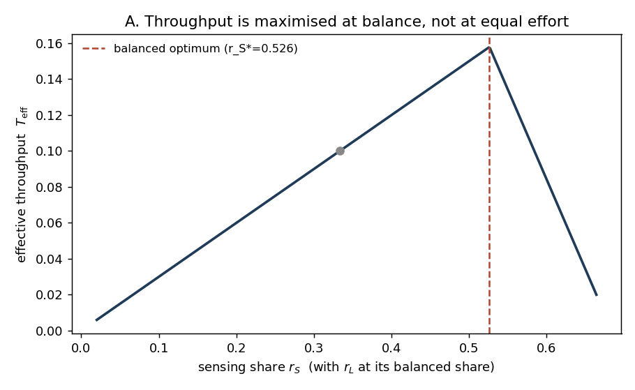
The first simulation confirms the corollary of §2.2: under a hypothetical fixed total capacity, effective throughput is maximised by equalising the efficiency-scaled stage rates rather than by equal effort. With a total capacity $R=1$ distributed across the three stages, a grid search over the allocation simplex locates the maximum of $T_{\text{eff}}=\min(\rho_{SL}\rho_{LE}\,r_S,\ \rho_{LE}\,r_L,\ r_E)$ at $(r_S, r_L, r_E)=(0.526,\,0.316,\,0.158)$, matching to three decimal places the analytic balance point at which all three scaled rates coincide. The throughput there is $T_{\text{eff}}=0.158$. An equal-effort allocation — a third of the total to each stage — yields $T_{\text{eff}}=0.100$: the balanced allocation delivers fifty-eight per cent more adaptive throughput from the same total, with no stage doing more work, only the work distributed to match the loop. The zero-marginal-return property is confirmed directly: starting from an execution-binding allocation and adding a further fifth of the total to the non-binding sensing stage moves $T_{\text{eff}}$ by exactly zero. [R within the model.] Capacity poured into a stage that is not the bottleneck does not accelerate adaptation; it is, in the dynamic terms of §2.2, converted to backlog rather than to throughput.

(Figure: xv_A_allocation.png — throughput along a one-dimensional slice through the optimum, with the balanced maximum and the lower equal-effort point marked.)

5.2 Simulation B — The Three Backlogs

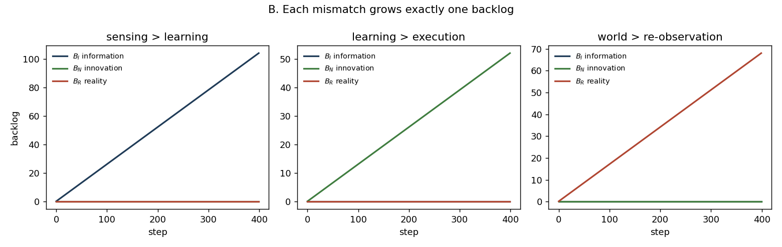
The second simulation runs the loop as an explicit queue model and confirms that each rate mismatch grows exactly one backlog while the others remain bounded. Three regimes were run. When sensing outruns learning ($r_S=0.60,\,r_L=0.10$), the information backlog $B_I$ grows linearly at 0.26 per step while $B_N$ and $B_R$ stay at zero. When learning outruns execution ($r_L=0.50,\,r_E=0.05$), the innovation backlog $B_N$ grows at 0.13 per step and the others stay flat. When world-change outruns re-observation, the reality backlog $B_R$ grows at 0.17 per step alone. [R within the model.] The three failure signatures of Part III are thus separable: each is the accumulation behind one specific leg, and a system can be diagnosed by which of its backlogs is growing.

The third regime required a detail that is itself a result worth recording. In the model, world-change from the controller's own execution is $g\cdot\tilde r_E$, where $g$ represents the amplification of an action's consequences beyond its immediate footprint — leverage, in the financial register of §1.1. With no amplification ($g=1$) and no exogenous disturbance, the reality backlog cannot grow at all, because the loop's own execution rate is bounded by $\tilde r_E \le \rho_{SL}\rho_{LE}\,r_S = 0.30\,r_S < r_S$: a system's unamplified action can never outrun its own sensing, since the conversion losses guarantee that less reaches the world than the sensing stage took in. The reality backlog therefore has exactly three drivers, and raw busyness is not among them: a fast-changing world (large exogenous $d$), action whose consequences are amplified beyond their footprint ($g>1$), or — the case Simulation D isolates — sensing capacity diverted onto one target while the consequences of action accrue unobserved elsewhere. This sharpens the "execute less" remedy of §2.1: throttling execution relieves a reality backlog only to the extent that execution, through amplification, is what is outrunning re-observation; against a fast-changing world it does nothing, and only sensing capacity or a narrower boundary will serve.

(Figure: xv_B_backlogs.png — three panels, one per regime, each showing a single backlog growing.)

5.3 Simulation C — The Recursion Pulls Throughput Below the Minimum

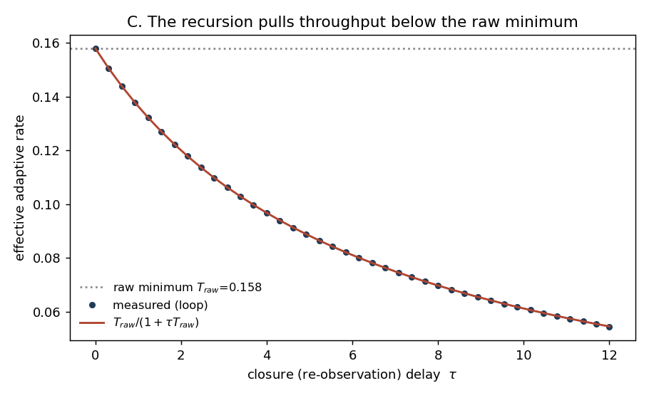
The third simulation establishes the recursion-specific result that §2.5 deferred. The raw stage-limited throughput of the loop — the rate at which an open, feedforward pipeline with these rates would deliver adaptation — is $T_{\text{raw}}=0.158$, the binding scaled rate from Simulation A. But the loop is not open: a corrective cycle cannot be fully informed until the previous execution's effects have been re-observed, a delay $\tau$ later. Sweeping the closure delay and measuring the rate at which completed adaptive cycles accrue, the simulated rate falls below $T_{\text{raw}}$ and matches the closed form

$$T_{\text{eff}}^{\,\text{rec}} = \frac{T_{\text{raw}}}{1 + \tau\,T_{\text{raw}}}$$

to within machine precision (maximum residual $\sim 3\times10^{-17}$ over $\tau\in[0,12]$). [R within the model.] The form was recovered from the loop, not assumed: it is what one obtains when each cycle costs a processing time $1/T_{\text{raw}}$ at the bottleneck plus a delay $\tau$ at the closure, so that the completion rate is $1/(1/T_{\text{raw}}+\tau)$. The throughput halves when $\tau = 1/T_{\text{raw}}$ — when the re-observation delay equals the bottleneck's own cycle time. This confirms the qualitative expectation of §2.5 with a specific dependence, and it gives the recursion its quantitative content: a governance loop with an able pipeline but a slow closure — a system that acts competently but re-observes the consequences of its action only after long delay — adapts at a rate strictly below what its stage capacities alone would suggest, and the shortfall is set entirely by the closure delay.

(Figure: xv_C_closure_delay.png — measured rate against $\tau$, with the closed form and the raw minimum overlaid.)

5.4 Simulation D — Effective and Self-Blinding

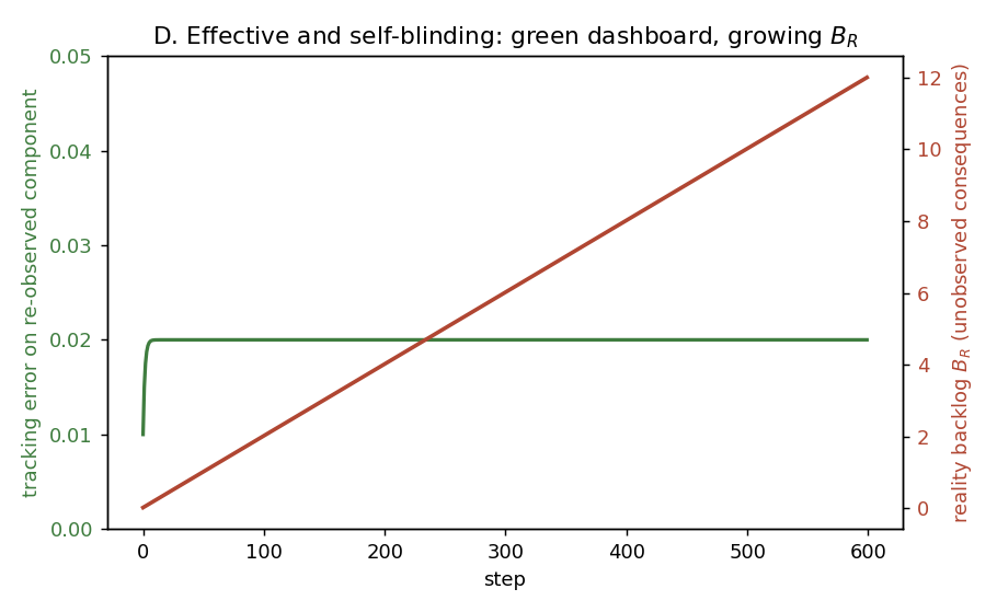
The fourth simulation isolates the case §2.4 named: a system in which execution is the binding stage but the loop still adapts faster than the environment drifts, so that the system tracks the component it re-observes while accumulating a reality backlog from the consequences it does not. The controller tracks a target drifting at $r_{\text{env}}=0.02$, and on that re-observed component it holds a steady tracking error of 0.020 — flat across the run, the picture of a system performing to specification. Meanwhile its own execution generates consequences at a rate its saturated sensing cannot capture, and the reality backlog $B_R$ climbs linearly to 12.0 over six hundred steps, a growth of 0.020 per step that the tracking metric never registers. [R within the model] for the dynamics; [IP] for the institutional reading. The two curves are the formal portrait of a system that is simultaneously effective and self-blinding: every measure it runs reports health, because every measure it runs is built on the component it still observes, while the gap between the world it is making and the world it is modelling grows unread. This is the structural kin of Self II's perceived-versus-true legitimacy gap, in which perceived self-trust holds steady while the true state it conceals erodes beneath it; here the concealment requires no self-deception, only a sensing capacity spent entirely on the target and none left for the wake.

(Figure: xv_D_self_blinding.png — flat tracking error on one axis, linearly growing reality backlog on the other.)

5.5 What the Simulations Do and Do Not Establish

The simulations establish that the bottleneck theorem, the three separable backlogs, the closure-delay law, and the effective-but-self-blinding regime are internally consistent and behave as Part II describes; the two quantities Part II left to simulation — the balanced-allocation optimum and the form $T_{\text{raw}}/(1+\tau T_{\text{raw}})$ — are now in hand. They establish nothing about any real governance system. The rates, the conversion efficiencies, the amplification factor, and the drift and delay parameters are stipulated, not measured; §2.4's admission stands, that no field instrument is offered for any of them. What the simulations confirm is that the formal grammar is coherent and that its central claims are not artefacts of a particular reading — that a system allocating capacity by equal effort leaves throughput on the table, that the three backlogs are diagnosable separately, that a slow closure depresses adaptation below the stage minimum, and that a system can pass every test it sets itself while losing contact with what its actions are doing. Whether any institution exhibits these signatures, and at what rates, is the work of the empirical phase, not of this paper.

(Simulation script: gae-simulator-v17-adaptation-bottleneck.py, seed 20260618.)

Part VI — Design Implications, and What the Series Does Next

6.1 Diagnose the Bottleneck, Do Not Maximise the Stages

The first implication is a discipline of attention, and it runs against the reflex of most reform. The reflex asks of each function whether there is enough of it — enough monitoring, enough analysis, enough delivery — and answers a shortfall by adding to the function that is visibly short. The bottleneck theorem says this is the wrong question. The right question is which single leg is binding, because capacity added to any other leg returns nothing: Simulation A's zero-marginal-return result is the formal statement that a system improving its non-binding stages is improving its self-assessment without improving its adaptation. [IP]. A governance system that wishes to adapt faster must find the one stage whose rate gates the loop and raise that, and it must resist the temptation to invest where investment is legible and measurable rather than where it binds — which are rarely the same place, since the binding stage is by definition the one whose output the rest of the system cannot use, and therefore the one that looks least productive from inside.

This redirects what a system should instrument. The metrics that each stage keeps of its own output — observations gathered, analyses produced, policies enacted — are exactly the metrics that cannot see the bottleneck, because each reports the stage doing its own job at full effort while the mismatch accumulates between stages (§3.4). The quantity that carries the diagnosis is the backlog: which queue is growing. A system adequate to its own adaptation watches the relations among its stage rates — the information, innovation, and reality backlogs — and reads its binding constraint off whichever is climbing, rather than reading a reassuring sum of stage outputs that no single dashboard can correct.

6.2 Relieve the Bottleneck by Functional Separation, Within a Limit

The worst architecture for the triad is the one that runs all three legs from a single pool of capacity, because there the fungibility of §4.1 turns against the system: the stages compete for the same attention, and the binding one is starved by whichever is most urgent or most rewarded. The structural remedy is functional separation — distinct subsystems carrying the three legs out of distinct, non-competing resources. The series has already named the pieces. Independent observers held apart from the pressures that correlate them are the sensing subsystem (Paper X). Protected experimental spaces, with exploration separated from exploitation and funded so the variance of learning is not extinguished by the incentives of delivery, are the learning subsystem (Paper XIV). The delivery apparatus is the executing subsystem (Papers IX, XI). Separation lets each stage's rate be raised without the others laying claim to the same resource, and it lets the reality-backlog remedy of §2.1 be applied locally — execution throttled in one domain where its consequences have outrun re-observation, without starving sensing across the whole architecture.

But separation is not free, and the model says exactly what it costs. Splitting the legs into subsystems lengthens the conversion legs between them: a model revision that once passed within a single body must now cross a boundary between bodies, and every such crossing is an attenuation of the kind Papers III and XI measured. Separation therefore raises the stage rates $r_S, r_L, r_E$ while lowering the conversion efficiencies $\rho_{SL}, \rho_{LE}$ that couple them — and since throughput depends on both, there is an interior optimum rather than a mandate to separate without limit. The design problem is to decouple enough that the stages stop starving one another, but not so much that the losses between subsystems consume what the decoupling bought. This is the bottleneck theorem's version of a tension the series meets elsewhere — the boundary trade-off of Paper XII, the depth cost of Paper XI — and it resolves the same way: by matching the degree of separation to where the binding constraint actually lies, not by maximising decoupling as a principle.

6.3 Instrument the Wake, Not Only the World

The recursion carries its own design implication, and it is the one most systems neglect because it is the one an open-pipeline intuition does not suggest. A system instruments the world it acts upon; far fewer instrument the consequences of their own action — the wake. Yet the reality backlog accumulates precisely there, on the leg where the system's execution returns to it as altered world, and a system that re-observes the conditions it inherited but not the conditions it created will read a model that is accurate about everything except what it is doing. Building the re-observation channel as a first-class element of the architecture — sensing capacity reserved for the effects of one's own action, not only for exogenous conditions — is the structural form of keeping the loop closed. The viability condition of §2.4 is the adequacy test for it: a system is keeping pace when its loop closes faster than the world drifts and its re-observation keeps abreast of what its own execution changes, $T_{\text{eff}} > r_{\text{env}}$ and $r_S \ge w$. Where the second condition fails, §2.1's bound says where to look — at amplification, at a fast-changing world, or at sensing spent entirely on the target with none left for the wake — and §6.2's separation says the remedy can be applied in the domain where the wake is going unread without dimming the system's sight elsewhere.

A curious consequence of the framework is that the reality backlog is not confined to governments. The architecture analysed in this paper is unusually general: a controller observes a world, forms a model of it, acts, and must then observe the consequences of its own action before acting again. Where execution persistently outruns re-observation, the controller's working model becomes progressively more a record of the world it inherited than of the world it has itself helped to create. The backlog accumulates most dangerously in the dimensions the controller assumes it already understands.

Nothing in this observation is specific to states or institutions. Organisations, firms, scientific communities, and individual persons all operate through adaptive loops of roughly the same form. The paper makes no claim that one ought therefore to spend more time reflecting, contemplating, or withholding action; those are normative questions outside its scope. It makes only the narrower structural claim that a system executing continuously without reserving capacity to re-observe its own wake eventually acts on a stale model, including a stale model of itself. If adaptation is the quantity of interest, then re-observation is not an interruption of the loop but one of its indispensable stages.

The point is deliberately modest. A controller may fail because it observes too little, learns too little, or executes too slowly. This paper adds that it may also fail because it mistakes the completion of an action for the completion of an adaptation. The loop does not close when the action is taken. It closes only when the consequences of that action have been brought back into observation and allowed to revise the model from which the next action will be chosen.

6.4 What the Series Does Next

With this paper the second cycle's internal logic is complete, and the shape of the completion is the dual it was built to be. The first cycle established that the static deficits of an architecture compound — that a system carrying several at once is worse than the sum of them, and cannot see this in its outputs (Paper V). The second cycle establishes that the dynamic capacities of an architecture bottleneck — that a system rich in two of the three adaptive rates is no faster than its slowest, and likewise cannot see this in its outputs. Compounding deficits and bottlenecked capacities are the two ways the parts of a multi-part architecture fail to be independent, and the series now holds one at each end of its two theoretical cycles. Nothing in this paper is a new primitive; it is the consolidation the second cycle had been pointing toward since the adaptation triad was first stated as three requirements that had never been costed together.

What remains is named and deferred in the same breath, on the discipline the series applies to itself. The interference version — the legs not queuing behind one another but disturbing one another — is the higher-order term this paper leaves open (§4.3), to be derived rather than borrowed if it can be made rigorous at all. The ecology of co-adapting architectures, where one controller's execution is another's disturbance and the loop analysed here is only one of many coupled together, is the natural next object (§4.4), and it waits by design: the single-controller claims should pass the empirical gate before a multi-controller theory is built on them. That is not a hedge but the framework keeping faith with its own first commitment — that a documented confrontation with data is worth more than an untested elaboration, and that the right response to an architecture meant to perceive more than any one vantage can is to hand the building of it to more vantages than one. The bottleneck is specified precisely enough to be measured. Whether any institution sits where the theory says it might is the work that this paper, having finished its own, leaves open for others to take up.

Appendix A — Formal Derivations

This appendix gives the derivations underlying Part II. It states the recursive lossy-loop model precisely, proves the bottleneck theorem and its zero-marginal-return corollary, derives the balanced-allocation optimum and its closed form, derives the closure-delay law that §2.5 deferred to simulation, proves the bound under which the reality backlog cannot arise from a system's own unamplified action, and restates the bottleneck in the variety terms of §2.3. Claims are tiered as within the model; the governance analogues that follow each result are interpretive, [IP], and argued in the body rather than established here.

A.1 The Recursive Lossy Loop

Let the three stage rates be $r_S, r_L, r_E \ge 0$, in units of work per unit time, and let the two interior conversion efficiencies be $\rho_{SL}, \rho_{LE} \in (0,1)$. The realised rates along the pipeline are nested minima — each stage processes no faster than its own capacity and receives no more than the previous stage delivers after conversion:

$$\tilde r_L = \min\!\big(\rho_{SL}\, r_S,\; r_L\big), \qquad \tilde r_E = \min\!\big(\rho_{LE}\, \tilde r_L,\; r_E\big). \tag{A.1}$$

The effective adaptive throughput is the realised execution rate, which by substitution is a single nested minimum of three positively scaled stage rates:

$$T_{\text{eff}} = \tilde r_E = \min\!\big(\underbrace{\rho_{SL}\rho_{LE}\, r_S}_{a},\; \underbrace{\rho_{LE}\, r_L}_{b},\; \underbrace{r_E}_{c}\big). \tag{A.2}$$

The closure leg carries no conversion. Execution changes the world at rate

$$w = g\,\tilde r_E + d, \qquad g \ge 1,\; d \ge 0, \tag{A.3}$$

where $d$ is the exogenous disturbance rate and $g$ is the consequence-amplification factor of §2.1. Re-observation proceeds at the sensing rate $r_S$, and the reality backlog accumulates as the unmet world-change:

$$\dot B_R = \max\!\big(0,\; w - r_S\big). \tag{A.4}$$

The sensing rate $r_S$ appears in both (A.2) and (A.4): it feeds the front of the loop and bounds re-observation at the close. This double occurrence is the formal content of the recursion and the source of every closure-specific result below.

A.2 The Bottleneck Theorem

Write $a = \rho_{SL}\rho_{LE}\,r_S$, $b = \rho_{LE}\,r_L$, $c = r_E$, so that $T_{\text{eff}} = \min(a,b,c)$ from (A.2).

Theorem A.1 (bottleneck). $T_{\text{eff}}$ is non-decreasing in each of $r_S, r_L, r_E$, and is strictly increasing in $r_i$ only when the scaled rate associated with $r_i$ is the unique minimiser of $\{a,b,c\}$. For any stage whose scaled rate is not the unique minimiser, $\partial T_{\text{eff}}/\partial r_i = 0$: capacity added there leaves the adaptive rate unchanged and is converted to backlog on the leg that receives it. [R within the model.]

Proof. Each of $a, b, c$ is a strictly increasing linear function of its own stage rate and constant in the other two. The minimum of a finite set of functions is differentiable wherever the minimiser is unique, with gradient equal to that of the active (minimising) function; the gradient with respect to any non-active argument is zero. Hence if $c < \min(a,b)$ — execution binding — then $\partial_{r_S} T_{\text{eff}} = \partial_{r_L} T_{\text{eff}} = 0$ and $\partial_{r_E} T_{\text{eff}} = 1$; symmetrically for the other binding cases. Non-negativity of each partial gives monotonicity. ∎

The surplus that the added capacity becomes is a backlog, located by (A.1). The information backlog on the Sense → Learn leg grows precisely when arrivals exceed learning capacity, $\rho_{SL} r_S > r_L$, equivalently $a > b$; the innovation backlog on the Learn → Execute leg grows when $\rho_{LE}\tilde r_L > r_E$; and the reality backlog grows by (A.4) when $w > r_S$. Adding capacity to a stage whose scaled rate is already above the minimum pushes more work onto the leg downstream of it without raising $T_{\text{eff}}$ — the formal statement that effort spent off the bottleneck is converted to queue rather than to throughput.

The result is the dynamic dual of the static compounding of Paper V: there the architecture's deficits enter a product, here its capacities enter a minimum. The minimum structure itself is the common content of the law of the minimum, queueing theory, and the theory of constraints; what is specific to the loop is the recursion of A.1 and the grounding of $\rho_{SL}, \rho_{LE}$ in the series' prior results.

A.3 The Balanced-Allocation Optimum

Consider the hypothetical fixed-total problem of §2.2:

$$\max_{r_S, r_L, r_E \ge 0} \; \min(a,b,c) \quad \text{subject to} \quad r_S + r_L + r_E = R. \tag{A.5}$$

Proposition A.2. The maximiser of (A.5) equalises the scaled rates, $a=b=c$, and is $$> r_S^\* = \frac{R}{1 + \rho_{SL} + \rho_{SL}\rho_{LE}}, \quad > r_L^\* = \rho_{SL}\,r_S^\*, \quad > r_E^\* = \rho_{SL}\rho_{LE}\,r_S^\*, >$$ with optimal throughput $$> T_{\text{eff}}^\* = \frac{R\,\rho_{SL}\rho_{LE}}{1 + \rho_{SL} + \rho_{SL}\rho_{LE}}. >$$ [R within the model.]

Proof. Suppose at a feasible point the scaled rates are not all equal; let $S$ be the set of stages achieving the minimum and let stage $j \notin S$. Since $j$ is not binding, $r_j > 0$ (a stage at zero rate would have scaled rate zero, hence be in the minimiser set), so a quantity $\varepsilon > 0$ of budget can be moved from $j$ to a binding stage. This strictly raises the scaled rate of the binding stage while leaving $j$ non-binding for $\varepsilon$ small, hence strictly raises $\min(a,b,c)$. Therefore no feasible point with unequal scaled rates is optimal, and the optimum satisfies $a=b=c$. Solving $a=b$ gives $r_L = \rho_{SL} r_S$; $b=c$ gives $r_E = \rho_{LE} r_L = \rho_{SL}\rho_{LE} r_S$; substituting into the budget yields $r_S^\*$, and $T_{\text{eff}}^\* = c = \rho_{SL}\rho_{LE} r_S^\*$. ∎

The optimum allocates more raw capacity to the upstream stages, $r_S^\* > r_L^\* > r_E^\*$, because each downstream stage need only match the attenuated flow that reaches it; equal effort across stages is therefore strictly suboptimal whenever $\rho_{SL}, \rho_{LE} < 1$. At the illustrative values $\rho_{SL}=0.6, \rho_{LE}=0.5, R=1$: $r_S^\*, r_L^\*, r_E^\* = 0.526, 0.316, 0.158$, $T_{\text{eff}}^\* = 0.158$, against $T_{\text{eff}} = 0.100$ at equal thirds — confirmed by grid search in Appendix B.

A.4 The Closure-Delay Law

The throughput (A.2) is the rate at which an open pipeline with these rates would deliver adaptation. The loop is not open: by the recursion of A.1, a corrective cycle cannot be informed until the previous execution's effects have been re-observed, a delay $\tau$ after they are produced. Under the strict-closure reading — the controller credits an adaptive cycle only once its predecessor's consequences have returned through (A.4), so that it does not act on un-re-observed change — the time to complete one informed cycle is the bottleneck processing time plus the closure delay, in series:

$$T_{\text{cycle}} = \frac{1}{T_{\text{raw}}} + \tau, \qquad T_{\text{raw}} \equiv \min(a,b,c).$$

The completed-cycle rate is the reciprocal, giving the closed form

$$T_{\text{eff}}^{\,\text{rec}} = \frac{1}{\,T_{\text{cycle}}\,} = \frac{T_{\text{raw}}}{1 + \tau\,T_{\text{raw}}}. \tag{A.6}$$

This is strictly below $T_{\text{raw}}$ for any $\tau > 0$, decreases monotonically in $\tau$, tends to $T_{\text{raw}}$ as $\tau \to 0$ and to $1/\tau$ as $\tau \to \infty$. It halves when $\tau = 1/T_{\text{raw}}$ — when the re-observation delay equals the bottleneck's own cycle time. Appendix B confirms (A.6) against the simulated loop to machine precision. The strict-closure reading is a modelling choice and the conservative one: if successive cycles may pipeline — a new correction begun before the previous one's consequences return — the depression is smaller, and (A.6) is then an upper bound on the loss. The reading appropriate to a controller that must not act on consequences it has not yet re-observed is the strict one.

A.5 The Endogenous Reality-Backlog Bound

Proposition A.3. With unamplified consequences ($g=1$) and no exogenous disturbance ($d=0$), the reality backlog cannot grow: $\dot B_R = 0$ for all rate allocations. [R within the model.]

Proof. From (A.1), $\tilde r_E = \min(\rho_{LE}\tilde r_L, r_E) \le \rho_{LE}\tilde r_L \le \rho_{LE}\rho_{SL} r_S$, using $\tilde r_L \le \rho_{SL} r_S$. Since $\rho_{SL}, \rho_{LE} \in (0,1)$, the product $\rho_{SL}\rho_{LE} < 1$, so $\tilde r_E < r_S$. With $g=1, d=0$, (A.3) gives $w = \tilde r_E < r_S$, and (A.4) gives $\dot B_R = \max(0, w - r_S) = 0$. ∎

The reality backlog therefore has exactly three sources, and raw activity is not among them. It grows only through a fast-changing world ($d$ large), consequences amplified beyond their footprint ($g>1$, so $g\tilde r_E$ may exceed $r_S$), or sensing capacity diverted onto one target so that the rate effectively available to re-observe the consequences of action is below the nominal $r_S$ — the case isolated in Simulation D, where the controller's sensing is fully consumed tracking a drifting target. The asymmetry of the two backlog remedies follows: lowering $\tilde r_E$ removes the backlog only when $g>1$ is its driver; against exogenous $d$ it does nothing, and only raising $r_S$ or narrowing the boundary so that fewer consequences fall outside re-observation will serve.

A.6 The Bottleneck in Variety Terms

Let $V_d$ be the disturbance variety the architecture faces, net of what its objective reaches, and let $V_S, V_L, V_E$ be the variety each stage can carry — the number of independent distinctions it can register, represent, or actuate. Requisite variety (Ashby) requires each stage to carry at least $V_d$ for the loop to absorb the disturbance. The inter-stage conversions attenuate variety as the efficiencies attenuate rate: only a fraction of sensed distinctions survive into the model, and only a fraction of modelled distinctions survive into action. The absorbable variety of the loop is therefore the minimum of the attenuated stage varieties,

$$V_{\text{loop}} = \min\!\big(V_S,\; \sigma_{SL} V_L,\; \sigma_{SL}\sigma_{LE} V_E\big),$$

with $\sigma_{SL}, \sigma_{LE} \in (0,1)$ the variety-theoretic counterparts of the rate efficiencies. [IP]. The bottleneck theorem in this currency reads: a loop absorbs disturbance variety equal to its least stage variety, however much variety its other stages command. This is the same Ashbyan requirement Paper IV located at the point of contact, here distributed across the three process stages rather than across space; the two are distinct axes of one requirement, and neither subsumes the other (§2.3).

Appendix B — Simulation Specification

This appendix specifies the simulation of Part V in full, sufficient for independent reimplementation. All experiments are deterministic given the seed; the script is gae-simulator-v17-adaptation-bottleneck.py, seed 20260618, with conversion efficiencies fixed at $\rho_{SL}=0.6, \rho_{LE}=0.5$ throughout. The efficiency values are illustrative: the results are structural in $\rho_{SL}, \rho_{LE} < 1$, and their magnitudes set the severity of a bottleneck, not its existence.

B.1 The Loop Model

The dynamic experiments (B and D) run the recursive loop as a discrete-time queue. At each step, with current backlogs $B_I, B_N, B_R$:

$$\begin{aligned} \text{(Sense}\to\text{Learn)}\quad & \alpha_L = \rho_{SL}\, r_S, \quad p_L = \min(B_I + \alpha_L,\, r_L), \quad B_I \leftarrow \max(0,\, B_I + \alpha_L - r_L); \\ \text{(Learn}\to\text{Execute)}\quad & \alpha_E = \rho_{LE}\, p_L, \quad p_E = \min(B_N + \alpha_E,\, r_E), \quad B_N \leftarrow \max(0,\, B_N + \alpha_E - r_E); \\ \text{(Execute}\to\text{Sense)}\quad & w = g\, p_E + d, \quad B_R \leftarrow \max(0,\, B_R + w - r_S). \end{aligned}$$

Here $p_L, p_E$ are the per-step processed (realised) learning and execution; the steady-state values reproduce $\tilde r_L, \tilde r_E$ of (A.1). The default disturbance is $d = 0.05$ and the default amplification $g = 1$ unless a regime sets otherwise.

B.2 The Four Experiments

A — Allocation optimum. With total $R = 1$, a grid search over the simplex $r_S + r_L + r_E = R$ (step $0.002$) maximises $T_{\text{eff}}$ of (A.2) and is compared to the analytic optimum of Proposition A.2. The zero-marginal-return property of Theorem A.1 is checked by adding $0.2$ to the non-binding sensing stage from an execution-binding allocation and confirming $T_{\text{eff}}$ is unchanged. A one-dimensional slice through the optimum is plotted (xv_A_allocation.png).

B — The three backlogs. Three regimes are run for 400 steps, each starving one stage relative to its upstream supply: sensing > learning ($r_S=0.60, r_L=0.10, r_E=0.40$); learning > execution ($r_S=0.60, r_L=0.50, r_E=0.05$); world > re-observation ($r_S=0.60, r_L=0.50, r_E=0.40, g=4$). The dominant backlog's growth slope (final value / steps) is recorded; the other two remain at zero (xv_B_backlogs.png).

C — Closure-delay depression. At the balanced optimum from A, the closure delay $\tau$ is swept over $[0,12]$ (40 points). The completed-cycle rate is measured from the loop and compared to the closed form (A.6); the maximum absolute residual is recorded (xv_C_closure_delay.png).

D — Effective and self-blinding. A controller tracks a target drifting at $r_{\text{env}}=0.02$ with correction gain $0.5$, sensing capacity $r_S=0.10$ fully consumed tracking the target, and execution generating unobserved consequences at $w = 0.12 > r_S$. The tracking error on the re-observed component and the reality backlog $B_R$ are recorded over 600 steps (xv_D_self_blinding.png).

B.3 Parameter Table

B.4 Verified Results

The simulations confirm the internal consistency of Part II and supply the two quantities the body deferred — the balanced optimum of A.3 and the closure-delay form (A.6). They establish nothing about any real governance system; every rate, efficiency, amplification, drift, and delay is stipulated, and §2.4's admission that no field instrument is offered stands in full.